R’s Geospatial Kaleidoscope:
Exploring Perspectives, Strengths, and Challenges
III Congreso & XIV Jornadas de Usuarios de R, Sevilla, Spain
2024-11-07
Disclaimer
The following perspectives are incomplete and subjective
I am happy to discuss them further – catch me after the talk!
Geographical Perspective
How to represent the real world with data?
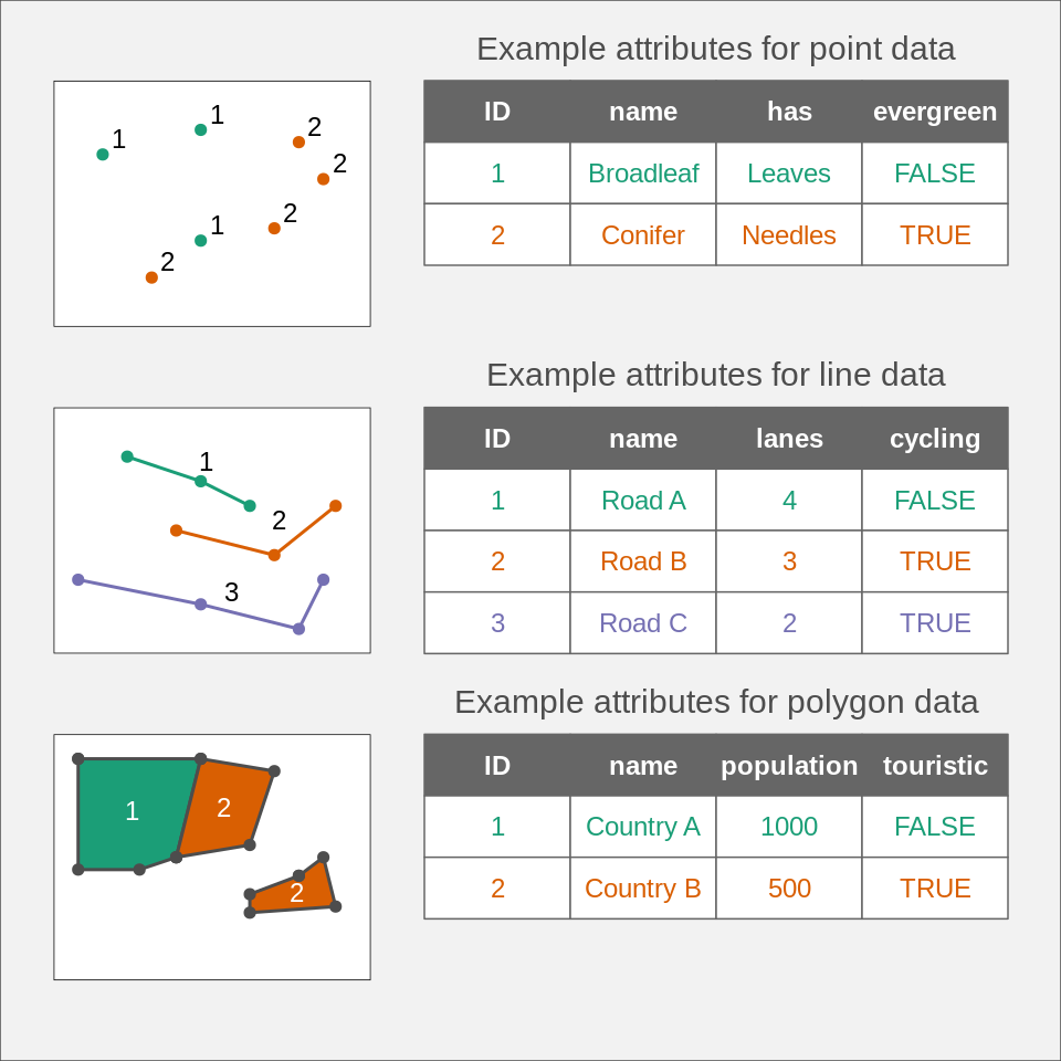
Vector data
Spatial vector data model: describing the real world as discrete objects
Simple features (sf) is an open standard developed and endorsed by the Open Geospatial Consortium (OGC)
Vector data

Source: https://r-tmap.github.io/
Vector data

Simple feature collection with 1 feature and 1 field
Geometry type: LINESTRING
Dimension:     XY
Bounding box:  xmin: 0.8 ymin: 1 xmax: 1 ymax: 1.2
Geodetic CRS:  WGS 84
# A tibble: 1 × 2
  id                       geom
  <chr>        <LINESTRING [°]>
1 1     (0.8 1, 0.8 1.2, 1 1.2)
Raster data
Spatial raster data model: describing the real world as continuous surfaces

Raster maps represent continuous phenomena such as elevation, temperature, population density or spectral data
They also can represent discrete features such as soil or land-cover classes
Raster data

Raster data
class       : SpatRaster
dimensions  : 1450, 1115, 1  (nrow, ncol, nlyr)
resolution  : 1000, 1000  (x, y)
extent      : 995456.5, 2110457, 4741961, 6191961  (xmin, xmax, ymin, ymax)
coord. ref. : NZGD2000 / New Zealand Transverse Mercator 2000 (EPSG:2193)
source      : nz_elev.tif
name        : elevation
min value   :     0.000
max value : 4140.333 
Other types of spatial data
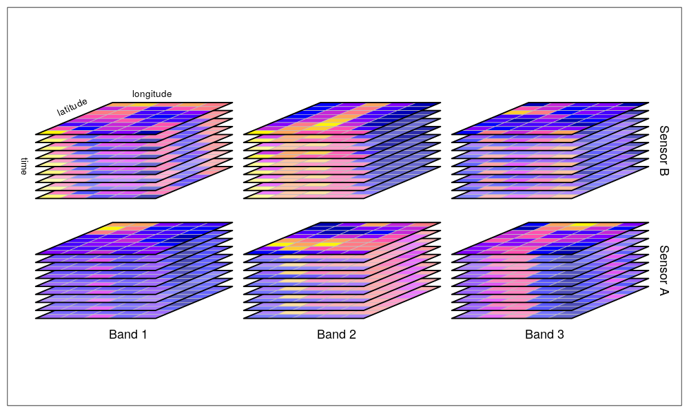
Data cubes/Spatiotemporal Arrays: https://r-spatial.github.io/stars/
Meshes: https://rpubs.com/cyclemumner/mdsumner-geomesh-foss4g
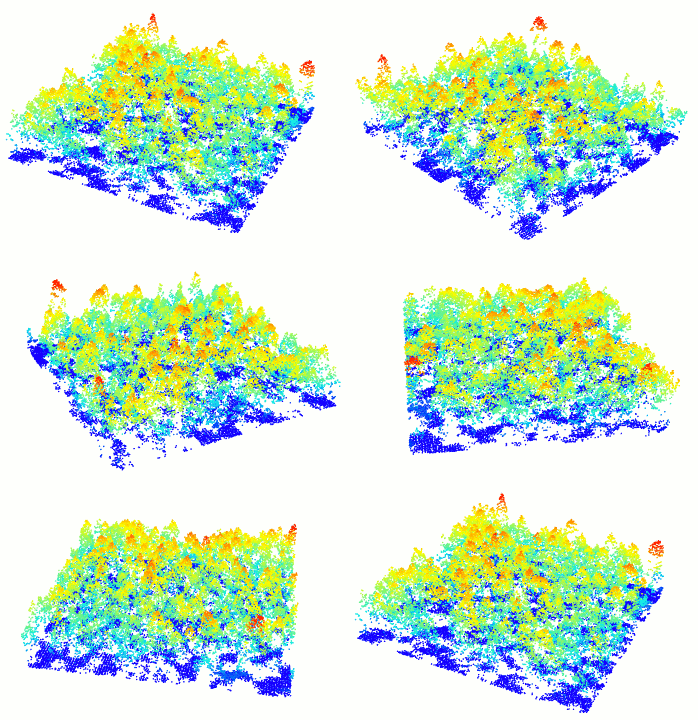
Point clouds: https://r-lidar.github.io/lidRbook/

Coordinate Reference Systems (CRSs)
Geographical coordinates

Projected coordinates


Coordinate Reference Systems (CRSs)
CRSs are crucial for spatial data analysis:
- Data integration
- Data visualization (map making)
- Spatial operations: distance, area, etc.

Statistical Perspective
Spatial statistics
Spatial statistics is a branch of statistics that explicitly takes location into account when describing and drawing inferences about the data.
Analysis type | Goal |
|---|---|
Point pattern analysis | Understand the spatial distribution of points |
Network analysis | Understand the spatial relationships between objects |
Geostatistics | Understand the spatial variation of a continuous variable, with interpolation being a common task |
Areal data analysis | Understand the spatial variation of a variable aggregated over areas |
Spatial statistics relation to spatial data
Spatial statistics is a branch of statistics that explicitly takes location into account when describing and drawing inferences about the data.
Analysis type | Data types |
|---|---|
Point pattern analysis | Points, polygons (observation window), raster (e.g., density estimation) |
Network analysis | Lines (creating a network), points (nodes and edges) |
Geostatistics | Points (with values), raster (e.g., the interpolation or simulation results) |
Areal data analysis | Polygons (with values), neighborhood lists, weight lists |
Spatial statistics
Data types conversion exist in many R spatial statistics packages
spatstat:
sfnetworks:
spdep:

Many statistical techniques make the assumption that observations are independent.

This assumption can be easily violated when working with ecological/environmental/geographical data.
Violation of this assumption can risk that the results will be wrong.
Temporal autocorrelation

Spatial autocorrelation

Spatial autocorrelation
The First Law of Geography:
“Everything is related to everything else, but near things are more related than distant things.”
—Tobler, 1970
…but, at the same time:
Autocorrelation may be found in the data also due to, for example, omitted variables or inappropriate levels of aggregation
Spatial autocorrelation
Friend or Foe?

What we want to achieve?
- Understand and describe the autocorrelation
- Draw inferences about the spatial processes
- Make predictions in unsampled locations
Describing spatial autocorrelation
library(tmap)
library(gstat)
data("lsl", "study_mask", package = "spDataLarge")
lsl_sf = st_as_sf(lsl, coords = c("x", "y"))
plot(lsl_sf["lslpts"], cex = 2)
plot(variogram(lslpts ~ 1, locations = lsl_sf))

Drawing inferences about spatial processes
Drawing inferences about spatial processes
Strategies when models’ residuals have spatial autocorrelation:
- Identify a non-random spatial process that can explain the autocorrelation
- Some people suggest aggregation of the data (but it seems not to be the best approach)
- Select a model that explicitly deals with autocorrelation, such as spatial lag or spatial error models (linear models that add a spatially lagged term to a linear regression model)
Spatial simultaneous autoregressive error model:
Drawing inferences about spatial processes
Making predictions in unsampled locations
Machine learning
The results of the hyperparameter tuning, feature selection, and (often) model evaluation depend on the selected cross-validation strategy.

Computational Perspective
File formats
Spatial data is stored in various file formats
Vector data:
- Shapefile (.shp): avoid if possible
- GeoPackage (.gpkg): better alternative
- GeoJSON (.geojson): good for web applications
- GeoParquet (.parquet): columnar storage format

Raster data:
- GeoTIFF (.tif): the most common format
- NetCDF (.nc): multidimensional raster data
- Zarr (.zarr): cloud-optimized format for multidimensional data
Point clouds:
- LAS (.las): the most common point cloud format
- LAZ (.laz): compressed version of LAS
File formats
A shapefile example
File formats
myurl = paste0("/vsicurl/https://zenodo.org/record/6211990/files/",
               "copernicus_DSM_100m_mood_bbox_epsg3035.tif") #~9.2 GB
dem = rast(myurl)
dem
class : SpatRaster
dimensions : 73590, 78430, 1 (nrow, ncol, nlyr)
resolution : 100, 100 (x, y)
extent : 869000, 8712000, -485000, 6874000 (xmin, xmax, ymin, ymax)
coord. ref. : ETRS89-extended / LAEA Europe (EPSG:3035)
source : copernicus_DSM_100m_mood_bbox_epsg3035.tif
name : copernicus_DSM_100m_mood_bbox_epsg3035
min value : -427025
max value : 5606973 
Cloud computing
Open big Earth Observation (EO) data availability has driven cloud computing solutions
Google Earth Engine (GEE):
- large user base
- well-designed API
- good for pixel-based raster processing of large EO data
Microsoft Planetary Computer (MPC):
- access to petabytes of EO data via STAC (“a catalog of spatiotemporal data”)
- providing access to MS Azure machines for data processing
- users can run their R/Python/Julia algorithms
Cloud computing
Open big Earth Observation (EO) data availability has driven cloud computing solutions
Google Earth Engine (GEE):
- free only (?) for non-commercial and research use
- (limited) API
- more complex types of analysis, such as object-based or time series analysis are hard or inneficient
Microsoft Planetary Computer (MPC):
- access to petabytes of EO data via STAC (“a catalog of spatiotemporal data”)
providing access to MS Azure machines for data processing(not anymore)users can run their R/Python/Julia algorithms(not anymore)
- rstac: connect, search, and download data from STAC catalogs
- gdalcubes: creates data cubes (consistent extent, resolution, etc.) from EO data
- sits: tools for time series analysis of EO data
- rsi: functions for downloading STAC data, calcularing spectral indices, and more
- openEO: a client for openEO API (a standard for processing EO data in different cloud environments)
- rgee: an R interface for Google Earth Engine
- (but still limited tools for image processing, spatial segmentation, or spatial deep learning)
Visual Perspective
Cartography
That was then…


R cartography
… and this is now
R (static) cartography
R (interactive) cartography

R cartography
A lot of developments in the last 10 years
At the same time, there seems to be many challenges and opportunities ahead – how to reimagine cartography using programming languages?
(Keep in mind to use the right tool for the right job)
Domain Perspective
Geospatial methods
Many geospatial methods are generalizable
- Exploratory data analysis (EDA)
- Output data in different formats (e.g., creating .GeoTIFF or .gkpg to share)
- Data processing (e.g. adding new variables)
- Data transformation (e.g., changing CRS)
- Spatial data analysis
- Data visualisation
- Web application development
- Software development e.g., to share new methdods
R spatial in various domains
Geospatial methods in R

Different domains use different terminologies
Reinventing the wheel is common
More collaboration accross domains is needed
The whole picture
The whole picture
Learn
A lot of resources are available: books, websites, and courses


Apply
Think if you can use R for your spatial data analysis: your domain expertise is crucial
Collaborate
Conversation is needed: learning from other successes and mistakes; learning from other fields


Extend
More people are welcome to the R spatial community: there are still many things to do
Learn
Apply
Collaborate
Extend
Contact
Mastodon: fosstodon.org/@nowosad
Website: https://jakubnowosad.com
Slides
http://jakubnowosad.com/IIIRqueR/


