

Using Moran’s I for assessing residual spatial autocorrelation in machine learning models
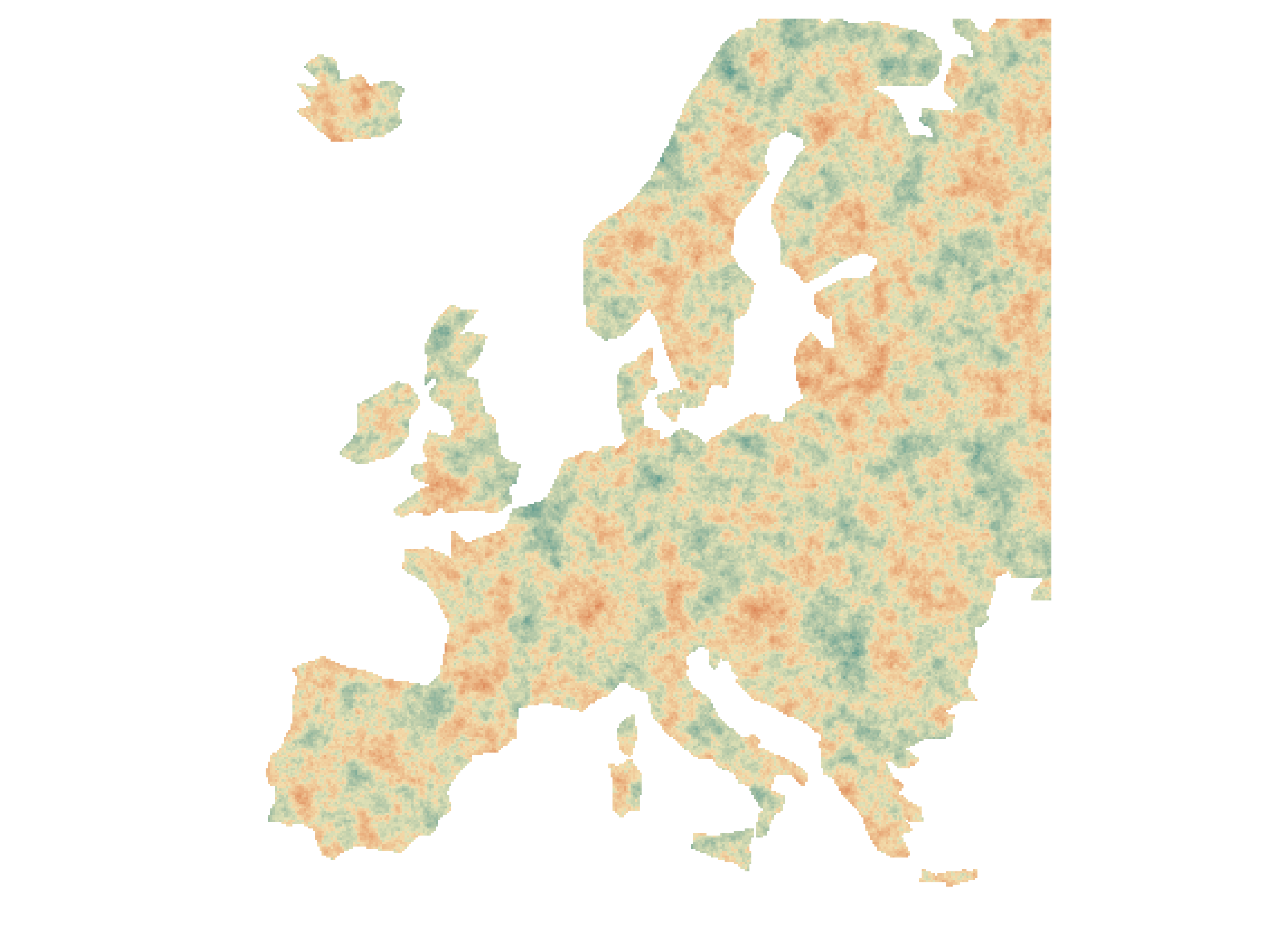
Same RMSE, different prediction maps
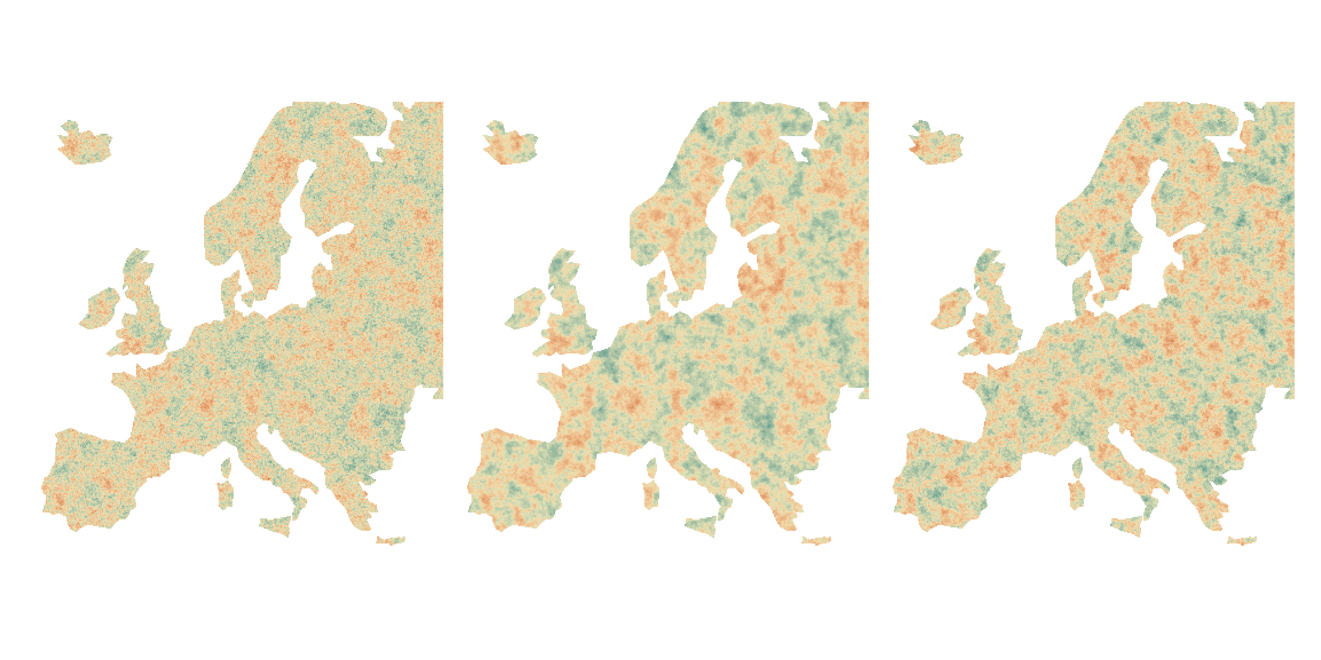
Residuals can still be spatially structured
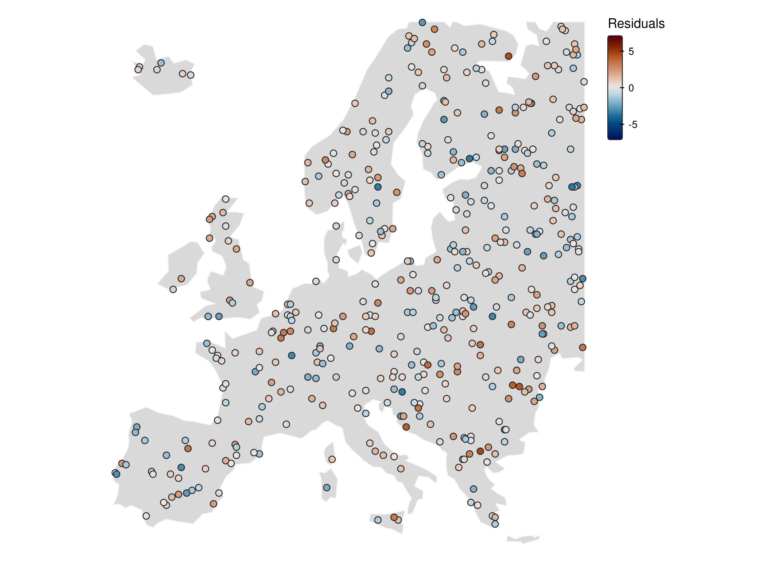
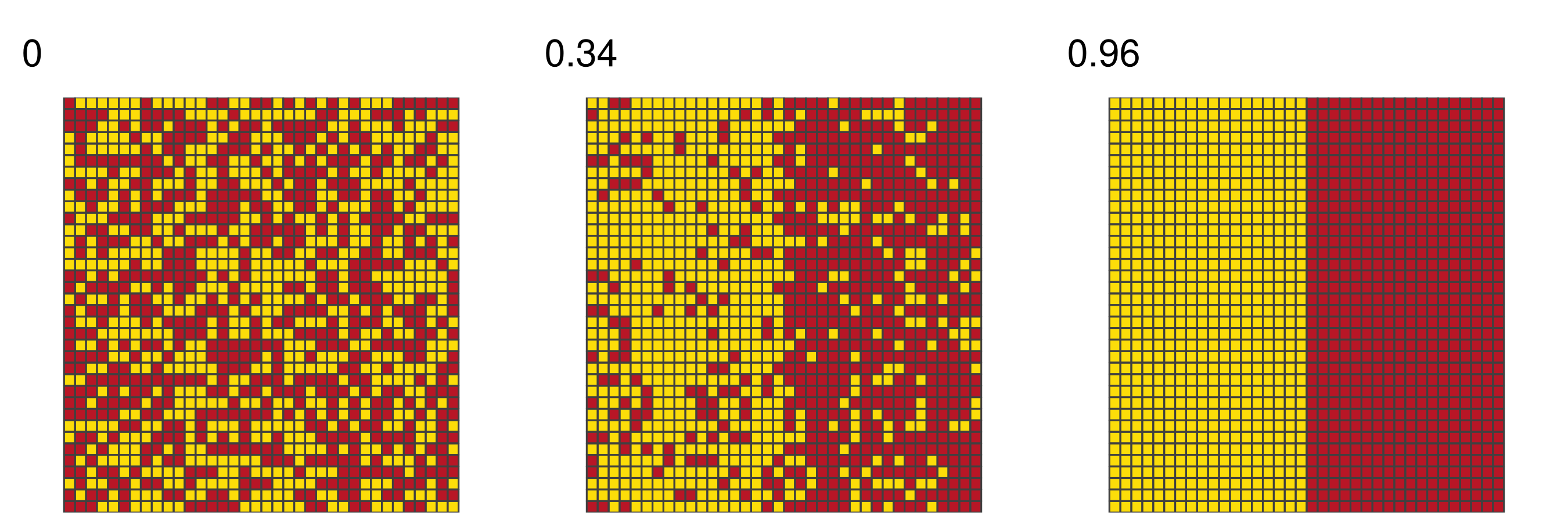
Moran’s I
Moran’s I measures similarity among neighboring residuals
\[ I = \frac{n}{\sum_{i}^{n} \sum_{j}^{n} w_{ij}} \times \frac{\sum_{i}^{n} \sum_{j}^{n} w_{ij} (x_i - \bar{x}) (x_j - \bar{x})}{\sum_{i}^{n} (x_i - \bar{x})^2} \]
- \(n\): number of observations
- \(x_i\), \(x_j\): values of the observations at locations \(i\) and \(j\)
- \(\bar{x}\): mean value of the observations
- \(w_{ij}\): spatial weight between the observations at locations \(i\) and \(j\)
Spatial weight defines which observations are considered neighbors.
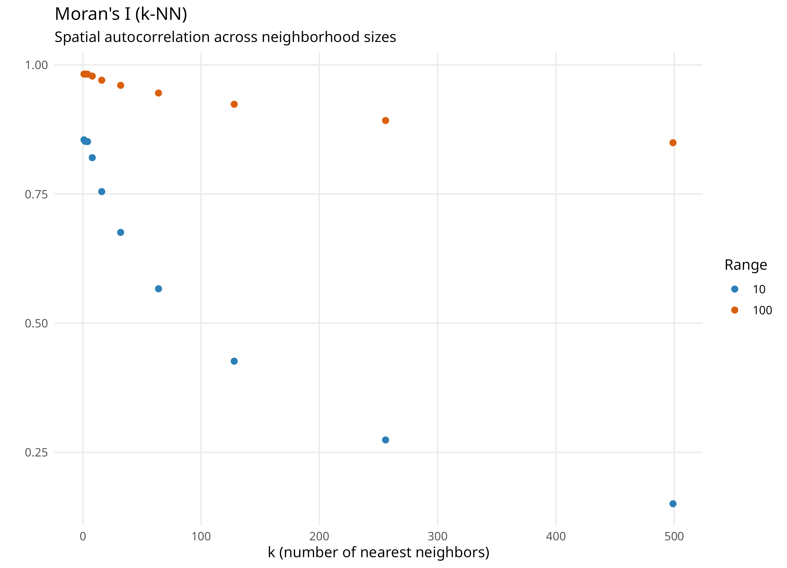
kNN-based weights
kNN: fixed number of neighbors, variable geographic extent
Larger k captures broader spatial structure
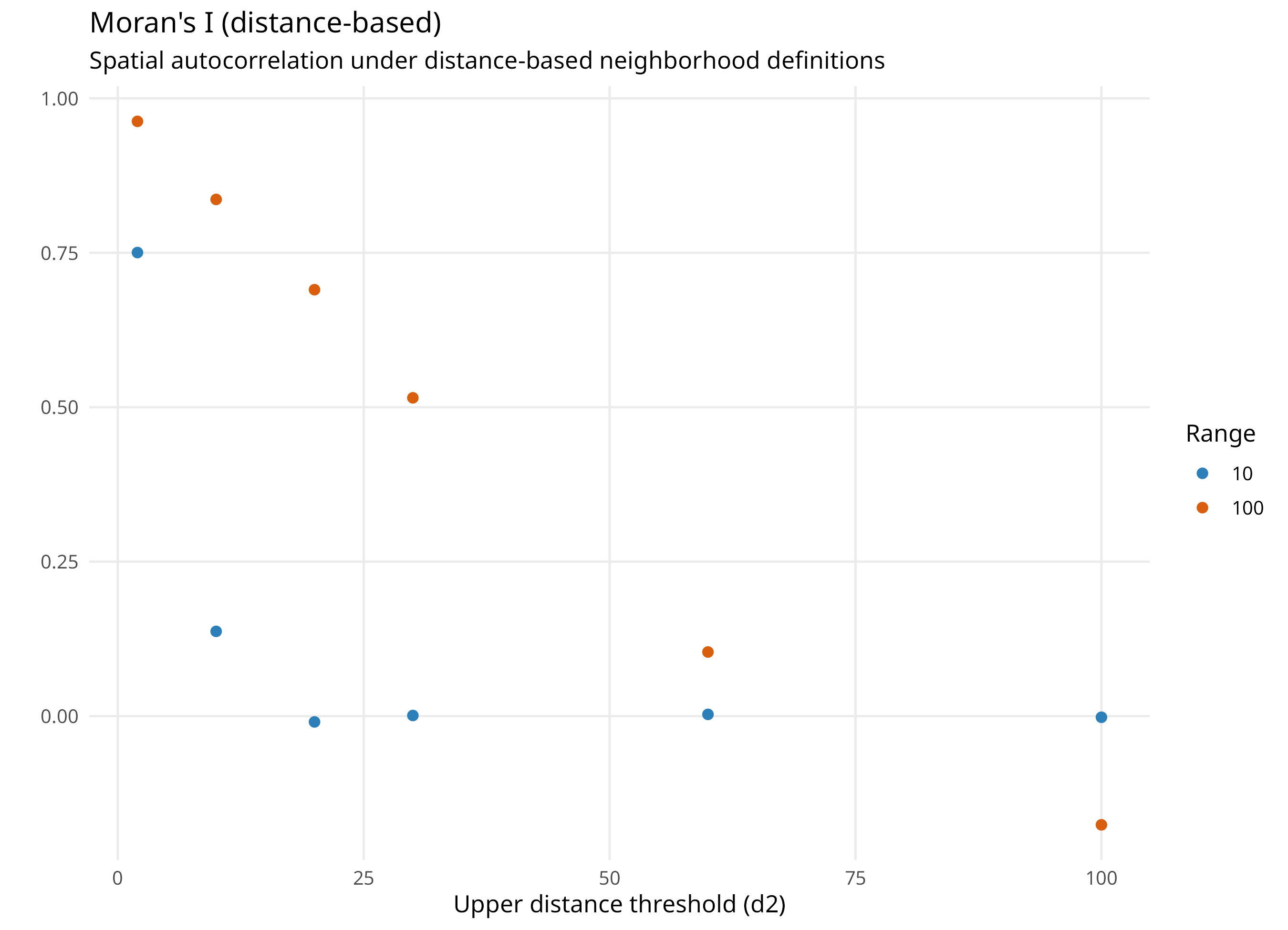
Distance-based weights
Distance-based: fixed geographic extent, variable number of neighbors
Smaller distance captures finer spatial structure, larger distance captures broader structure
Semivariogram
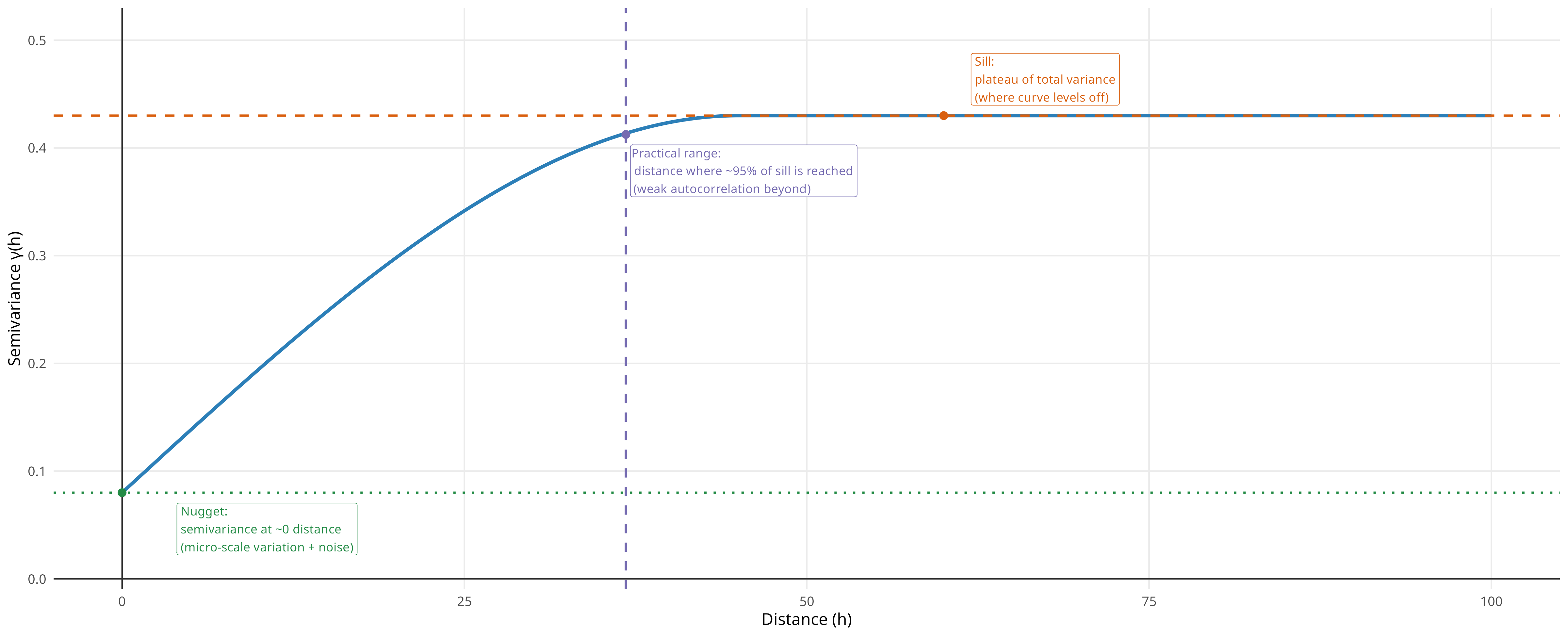
Semivariogram represents dissimilarity of observations as a function of distance, capturing spatial structure across distances
SSVR (Spatially Structured Variance Ratio)
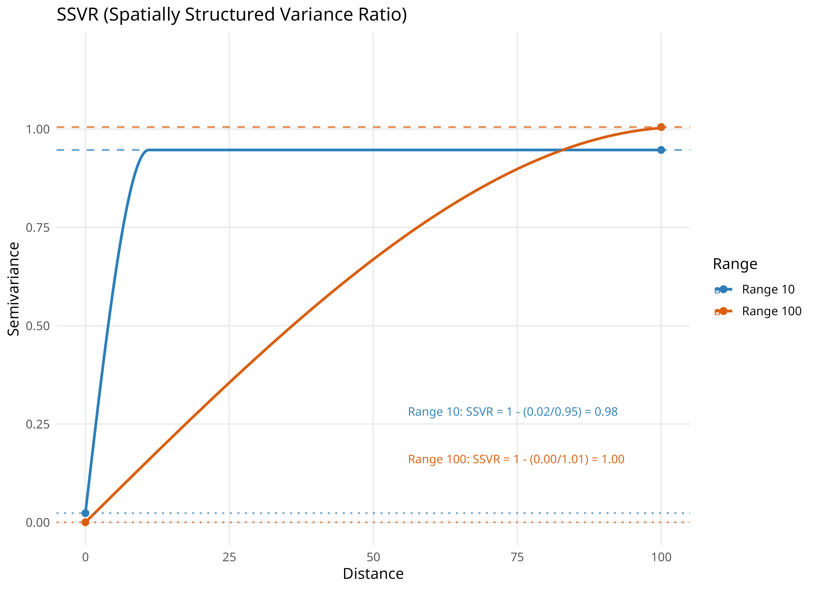
SSVR (Kerry and Oliver, 2008): share of spatially structured variance
An overall summary; ignores where in distance the structure occurs
Closer to 1 means stronger spatial structure
AUC (Area Under the Variogram Curve)
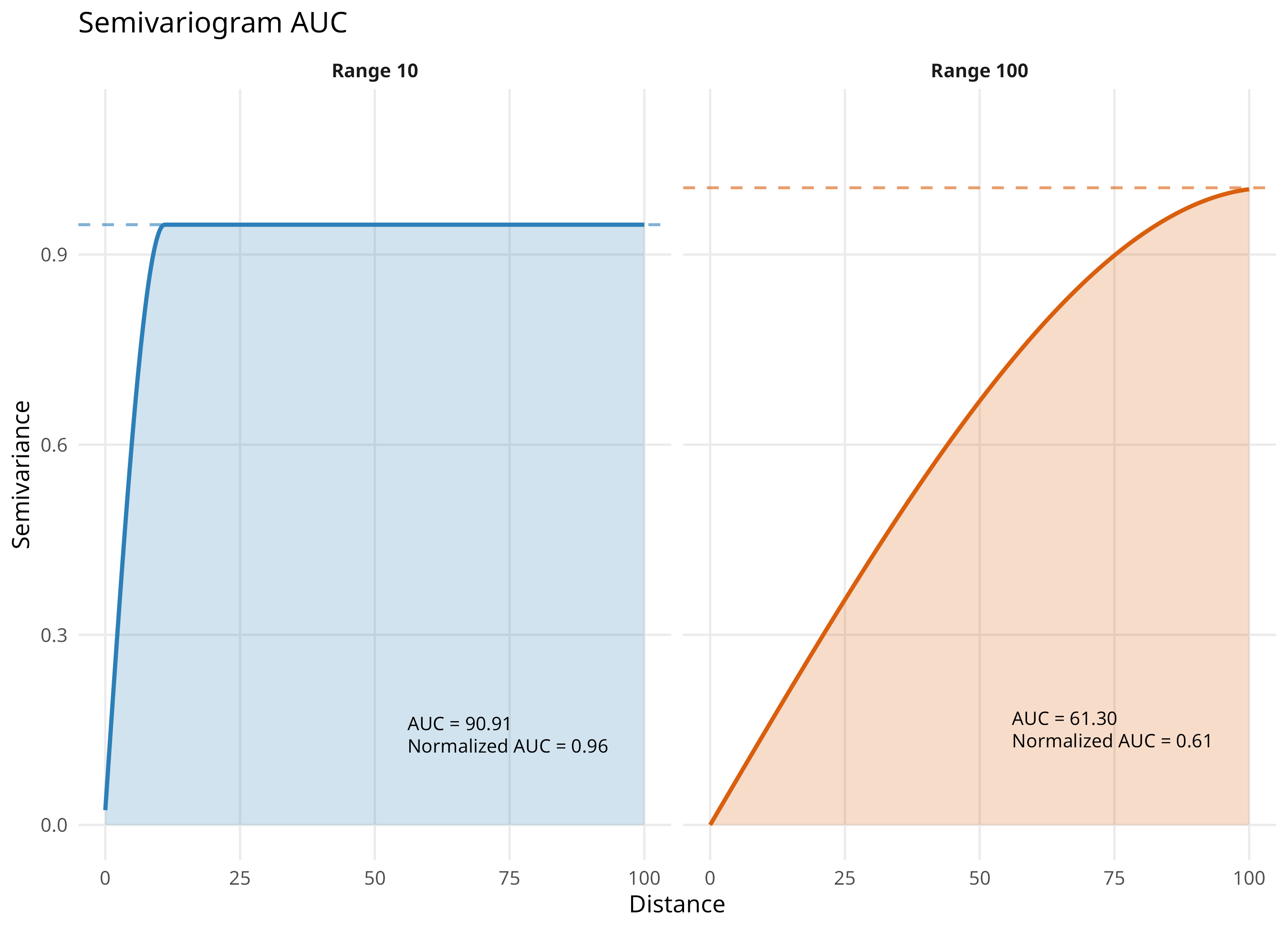
AUC of variogram (Poggio et al., 2019)
Integrates the spatial structure across distances, providing a single summary metric
Larger AUC values indicate stronger spatial dependence
- Integrates the variogram across distances
- Larger AUC values indicate stronger spatial dependence
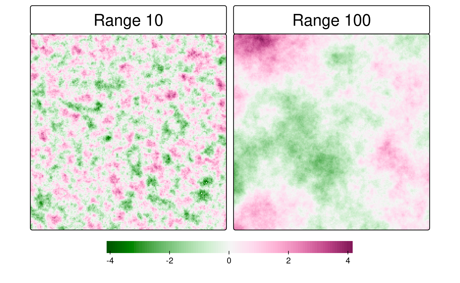
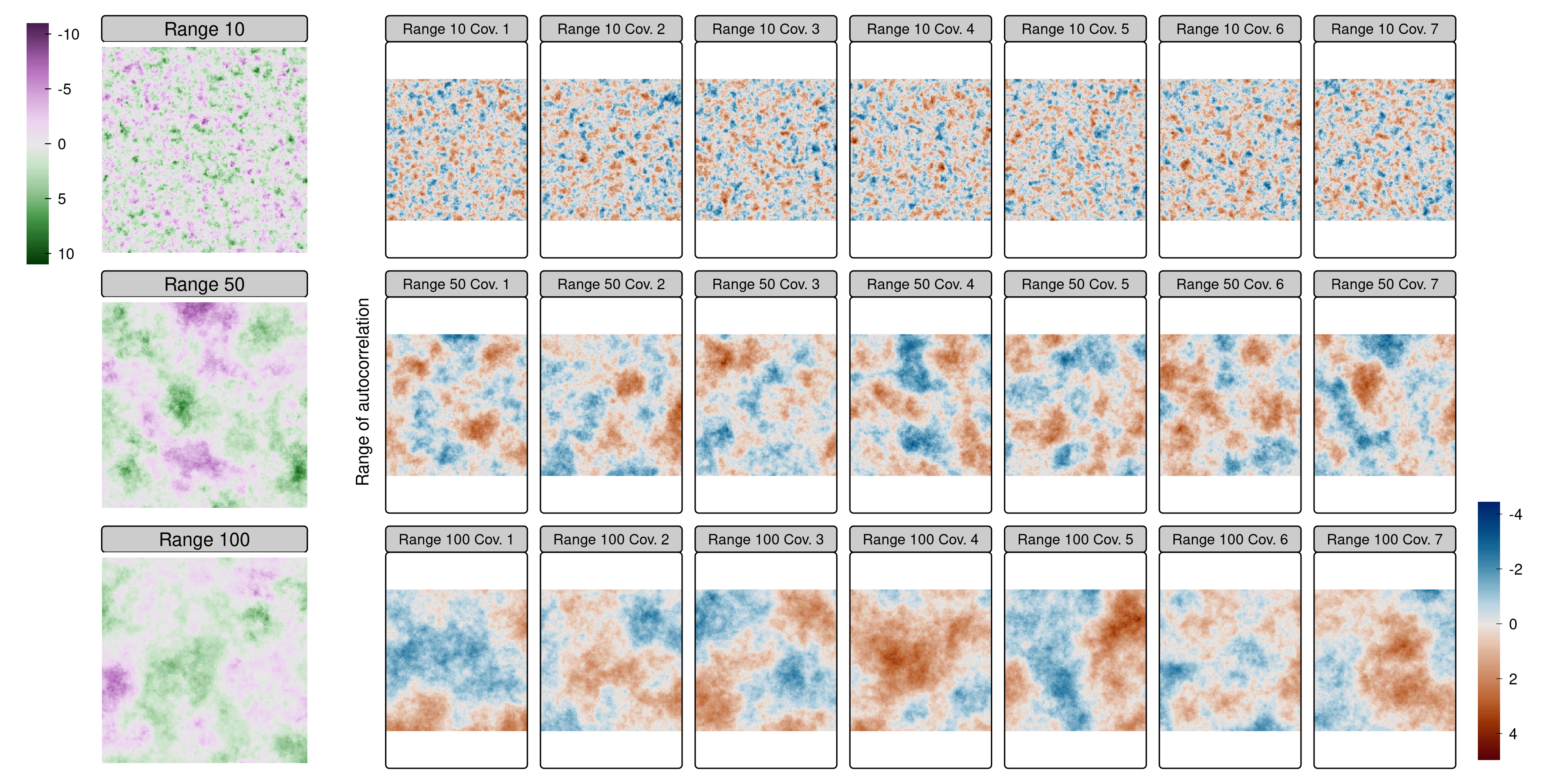
Simulation setup
Simulated rasters with three autocorrelation ranges (10, 50, 100 units)
Modeling setup
Random forest models fitted on samples of 500 points
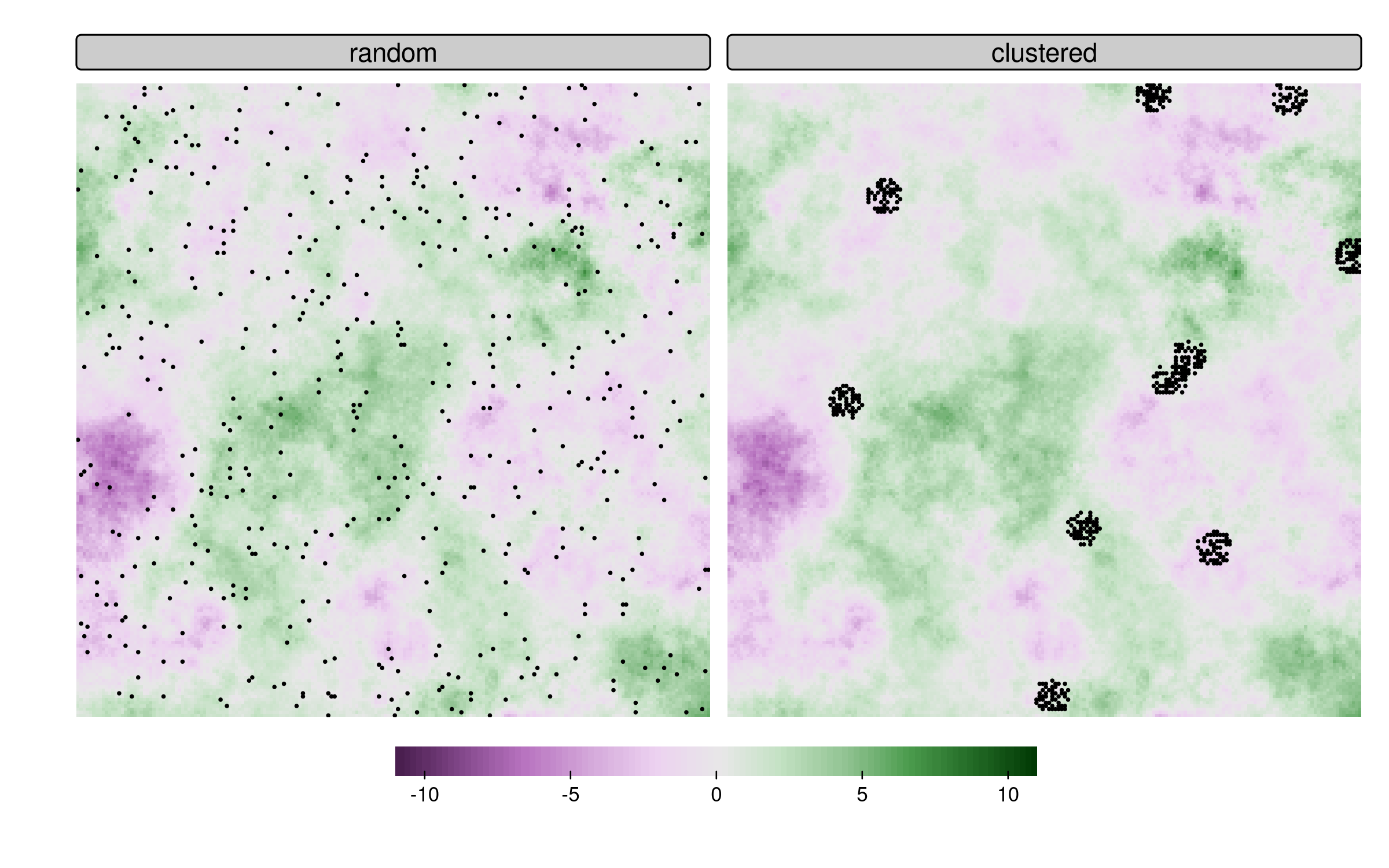
Validation setup
- Complete validation raster
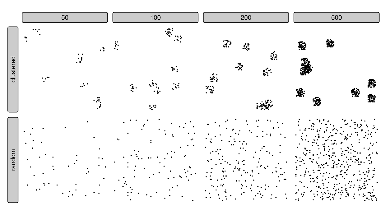
- Four test set sizes
- Two test set sampling types
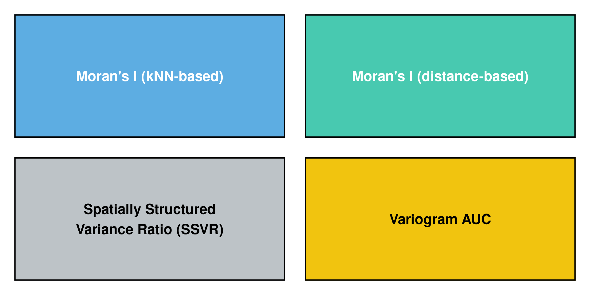
Diagnostic metrics:
- Moran’s I (kNN) (k=5)
- Moran’s I (distance) (from 0 to 100 units)
- SSVR
- AUC
- RMSE
\[ RMSE = \sqrt{\frac{1}{n} \sum_{i=1}^{n} (y_i - \hat{y}_i)^2} \]
Single example showcase
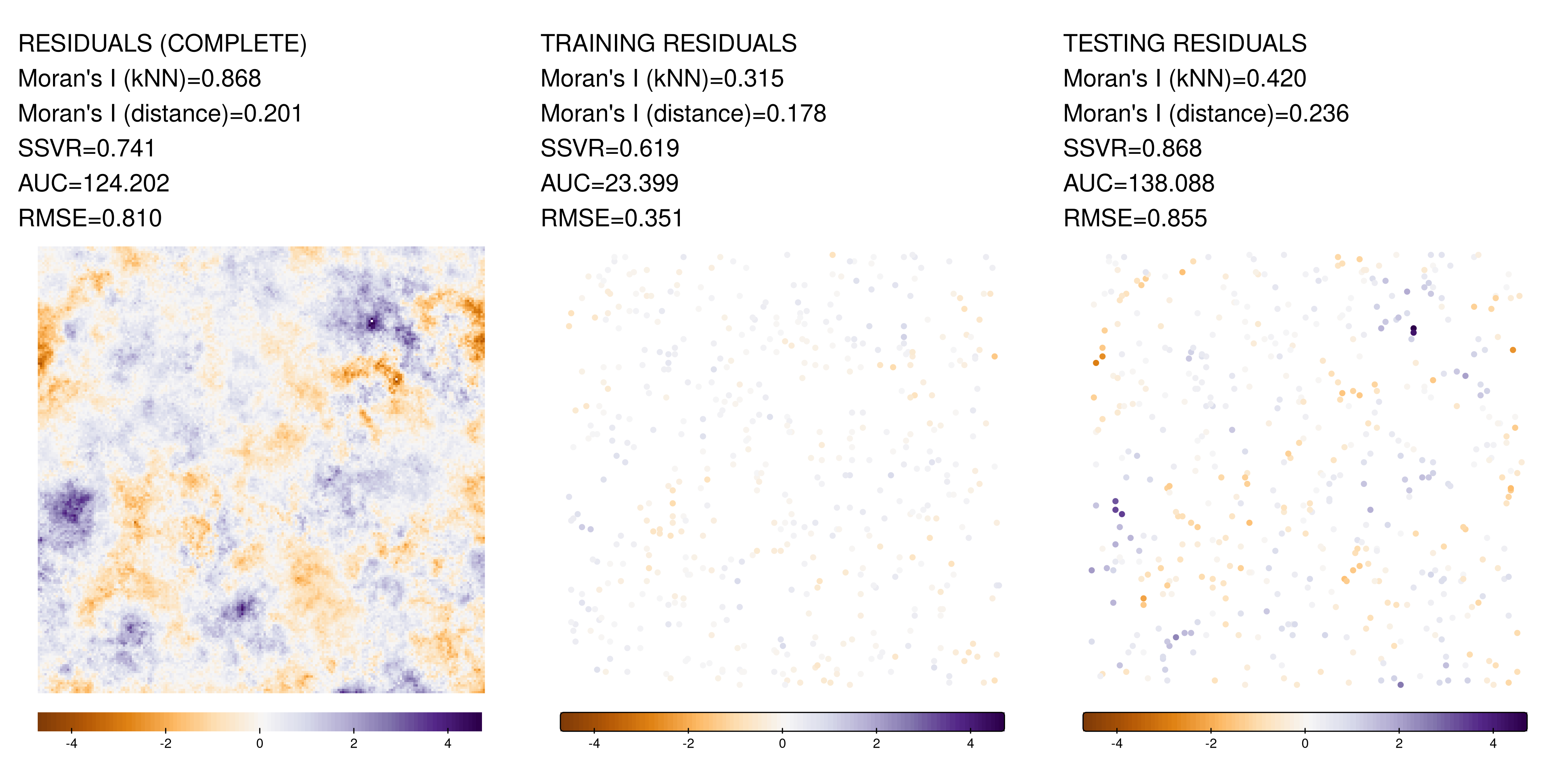
Relationship between metrics for different scopes
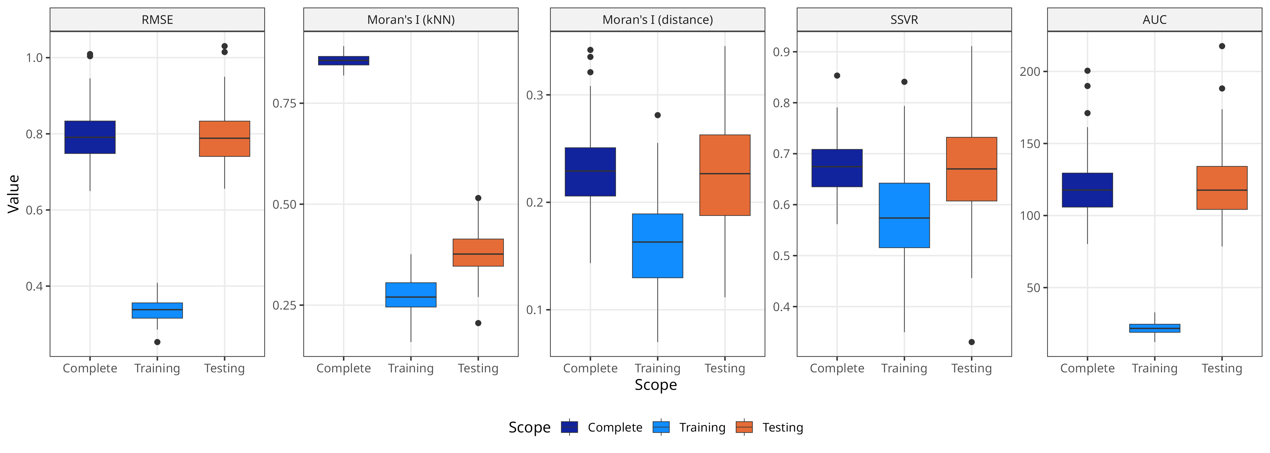
Metrics calculated on testing residuals are mostly comparable to those calculated on complete rasters
An exception is Moran’s I (kNN), with testing values much lower than complete values
Impact of test set size
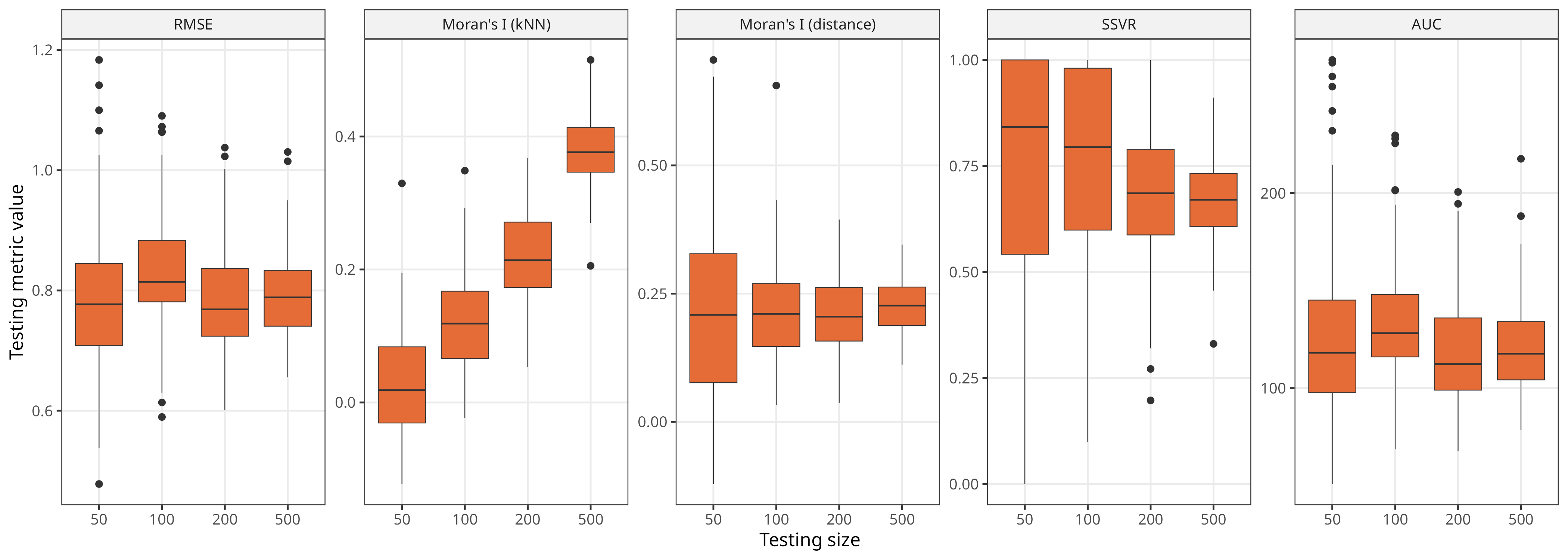
For most metrics, variability decreases as test set size grows, while mean values stay stable
Exception is again Moran’s I (kNN), which shows a strong increase in mean values with larger test set size
Random vs clustered sampling
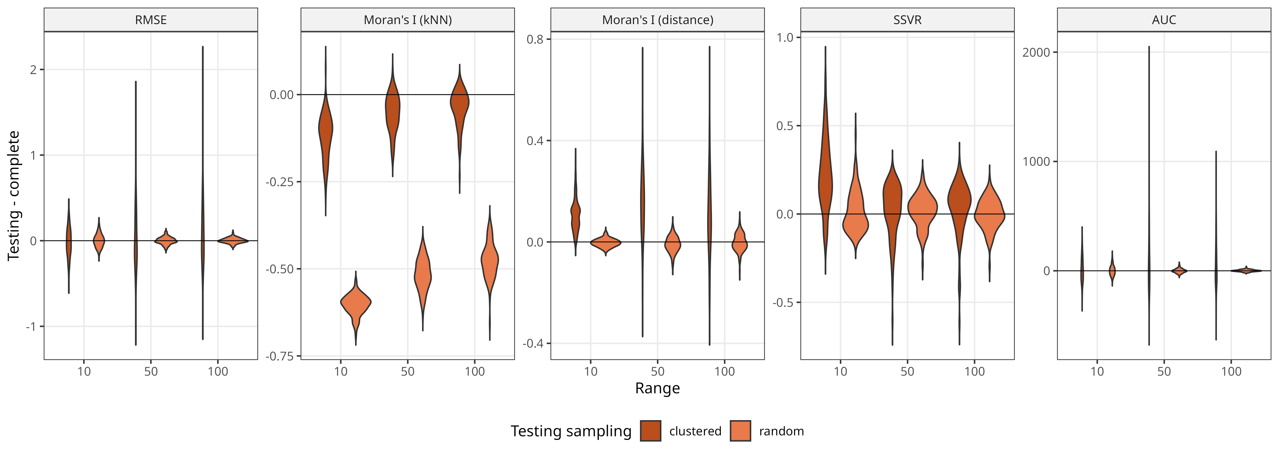
Clustered sampling affects all metrics, leading to higher variability and often incorrect mean values.1
Summary
- Assessing spatial autocorrelation in residuals is key for diagnosing model performance and understanding spatial structure in residuals
- Multiple metrics exist, each with different strengths and limitations
- They measure different aspects of spatial structure
- Report calculation parameters (e.g., k in kNN Moran’s I, distance thresholds) for transparency and reproducibility
Contact
Website: https://jakubnowosad.com
Resources
Slides: https://jakubnowosad.com/egu2026 Software: http://jakubnowosad.com/sacmetrics/

Take-home message
- Moran’s I examines autocorrelation at specific scales defined by the spatial weights
- SSVR summarizes the proportion of variance that is spatially structured
- Variogram AUC integrates spatial structure across all distances, closely tracking RMSE