Where can your spatial model be trusted?

Reliable validation of spatial machine learning
Jakub Nowosad (Adam Mickiewicz University, Poznań and University of Münster)

Earth Observation Summer School 2026, Istanbul, 2026-08-19

We often cannot measure the whole area of interest

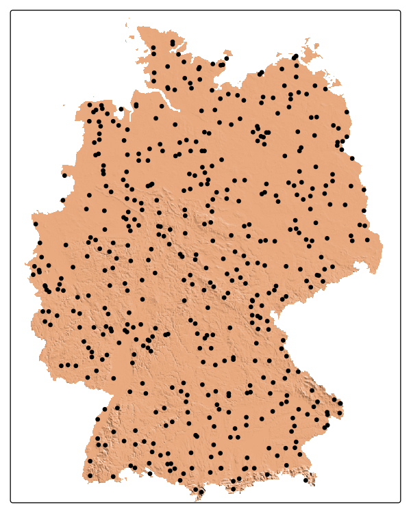
Extrapolation continuum

Predictive spatial machine learning

  • We have a limited number of observations, and several predictors that cover the whole area of interest (e.g., satellite imagery, elevation, climate, etc.)

Predictive spatial machine learning

  • We are interested in mapping across the spatial domain
  • Our goal is to forecast the future or map the present (not explain the model)
  • We train a model on the available observations and use it to predict across the whole area of interest
  • We then evaluate the model using a validation set
  • Thus, we should evaluate the map, not the model

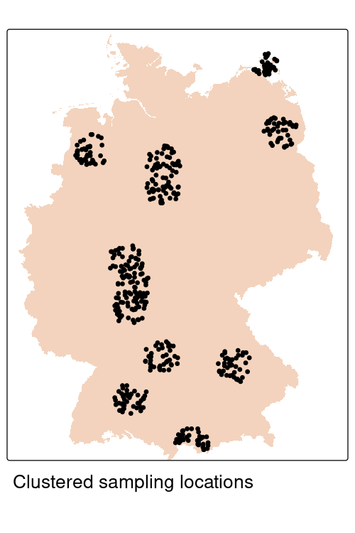
We validate where we have data, but predict where we do not

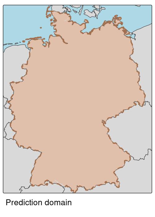
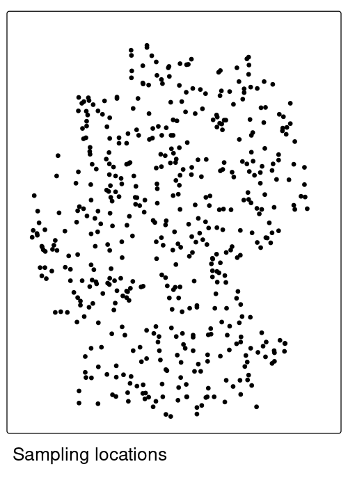
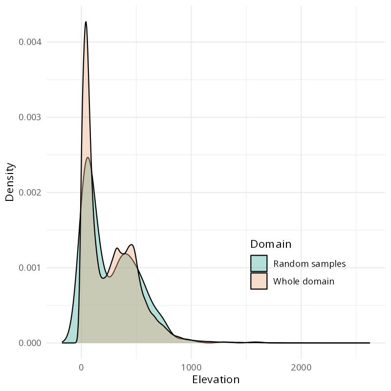
Similar application domain

We have this:

We want to predict here:

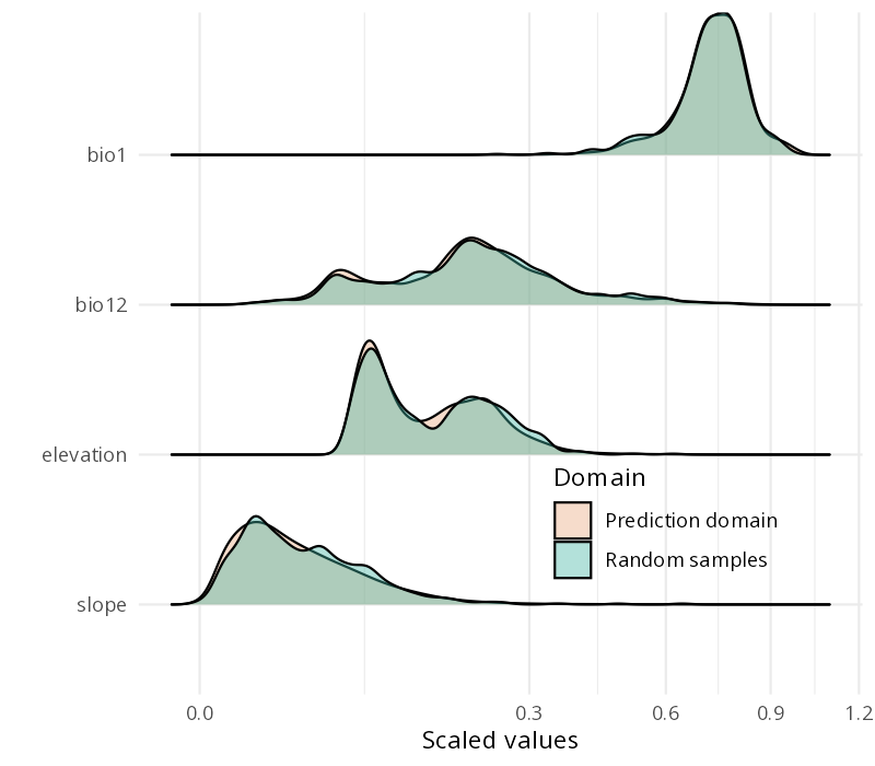
Similar application domain

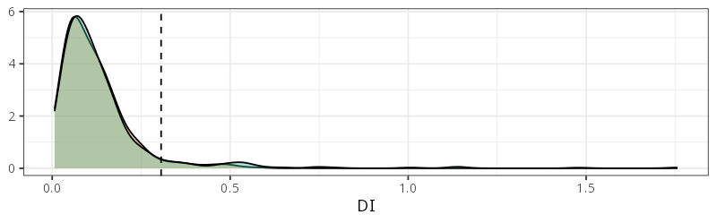
We have this:

Our predictor distributions are similar here:
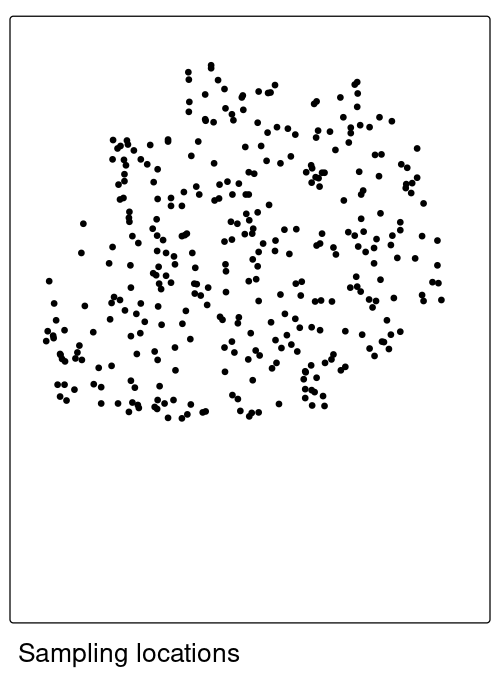
Different application domain

We have this:

We want to predict here:

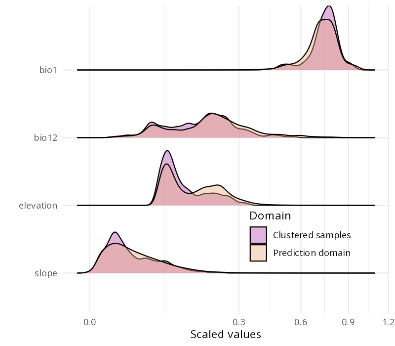
Different application domain

We have this:

Our predictor distributions are a bit different here:
Area of applicability

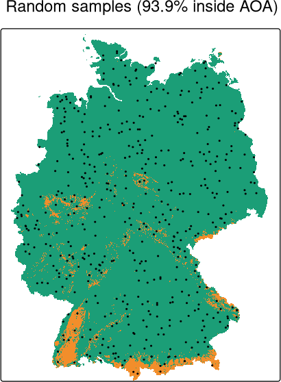
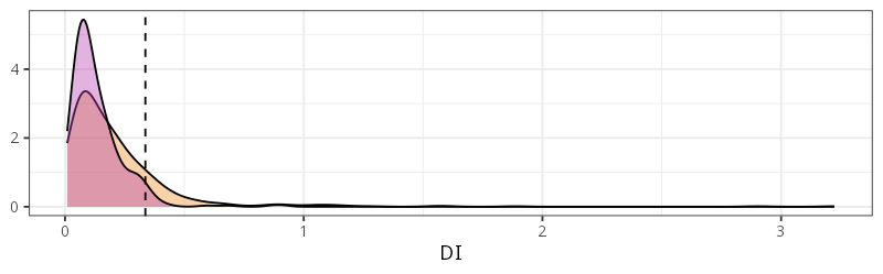
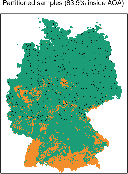
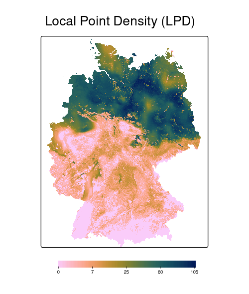
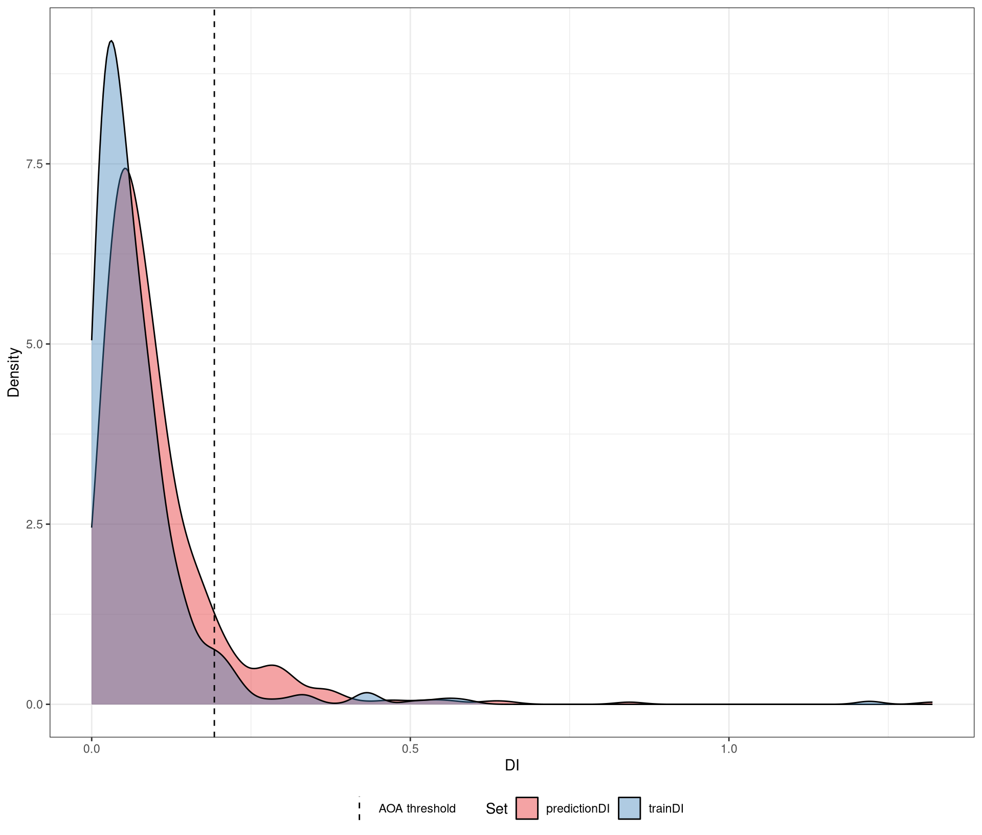
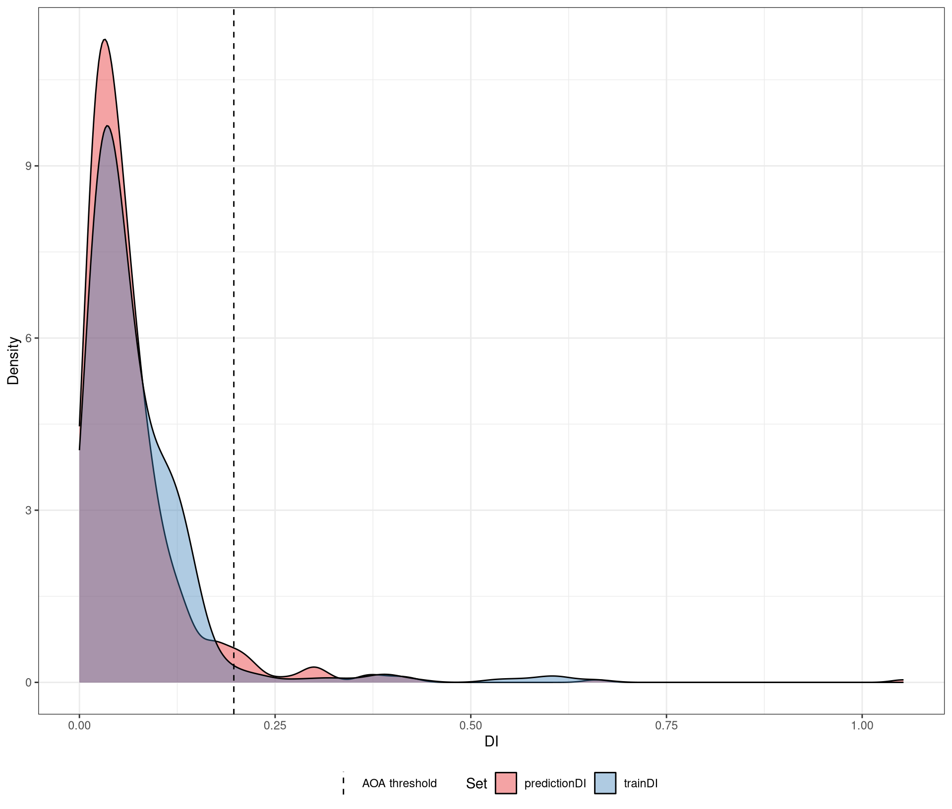
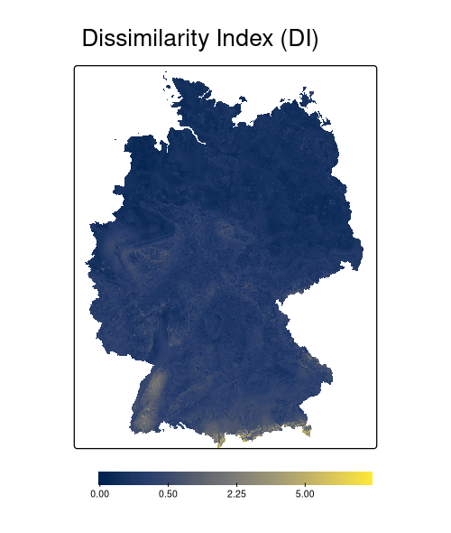
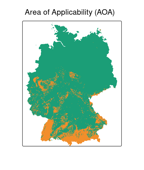
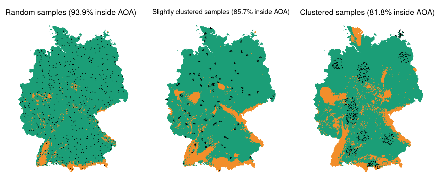
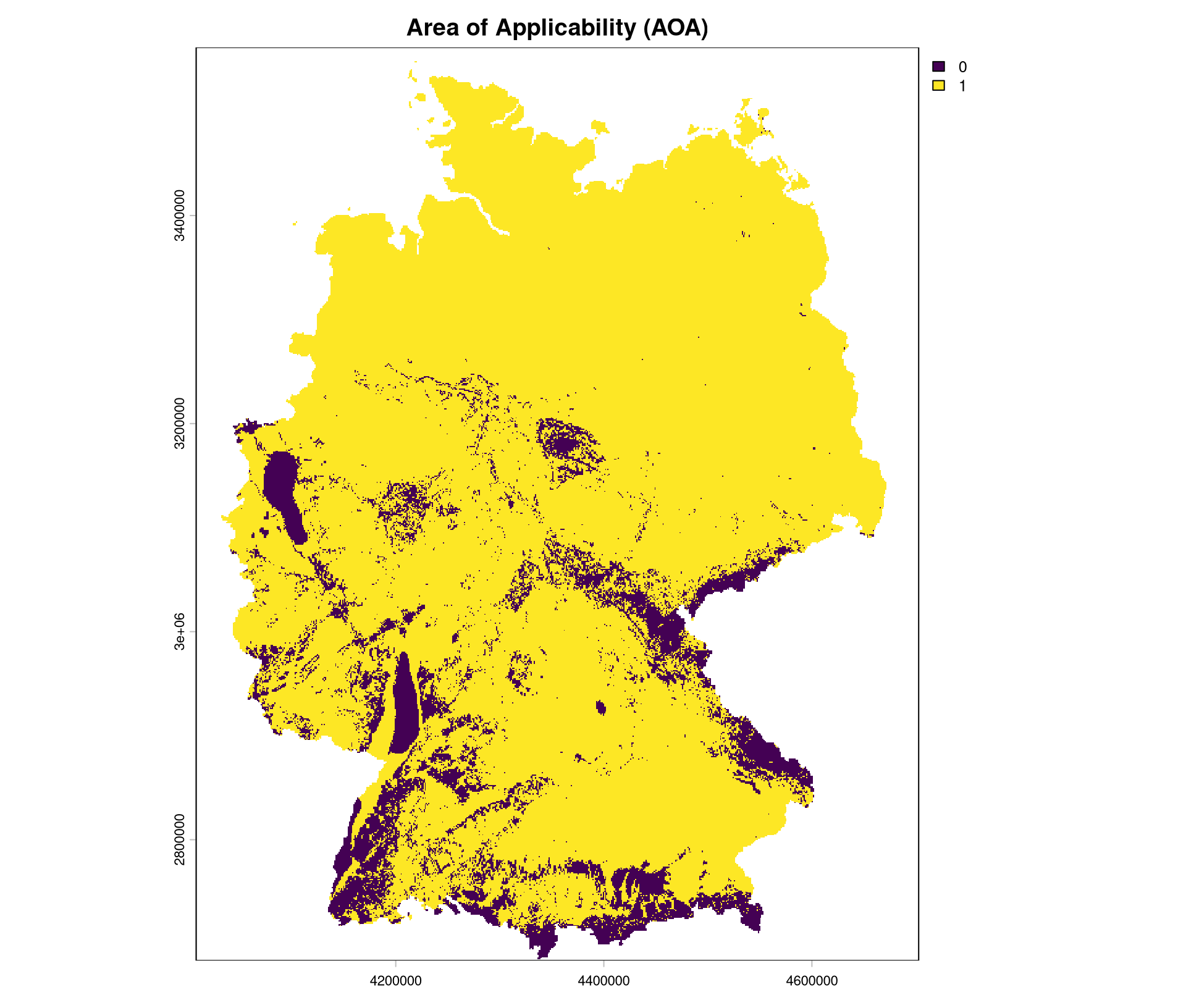
Identify areas where the environment is not well represented, making predictions less trustworthy (Area of Applicability – AoA, Meyer and Pebesma, 2021); also local point density (LPD, Schumacher et al., 2025)
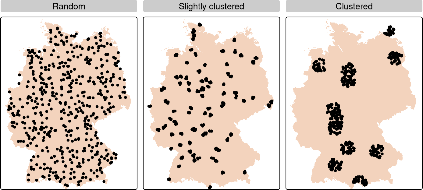
Area of applicability for different sampling designs
Examples

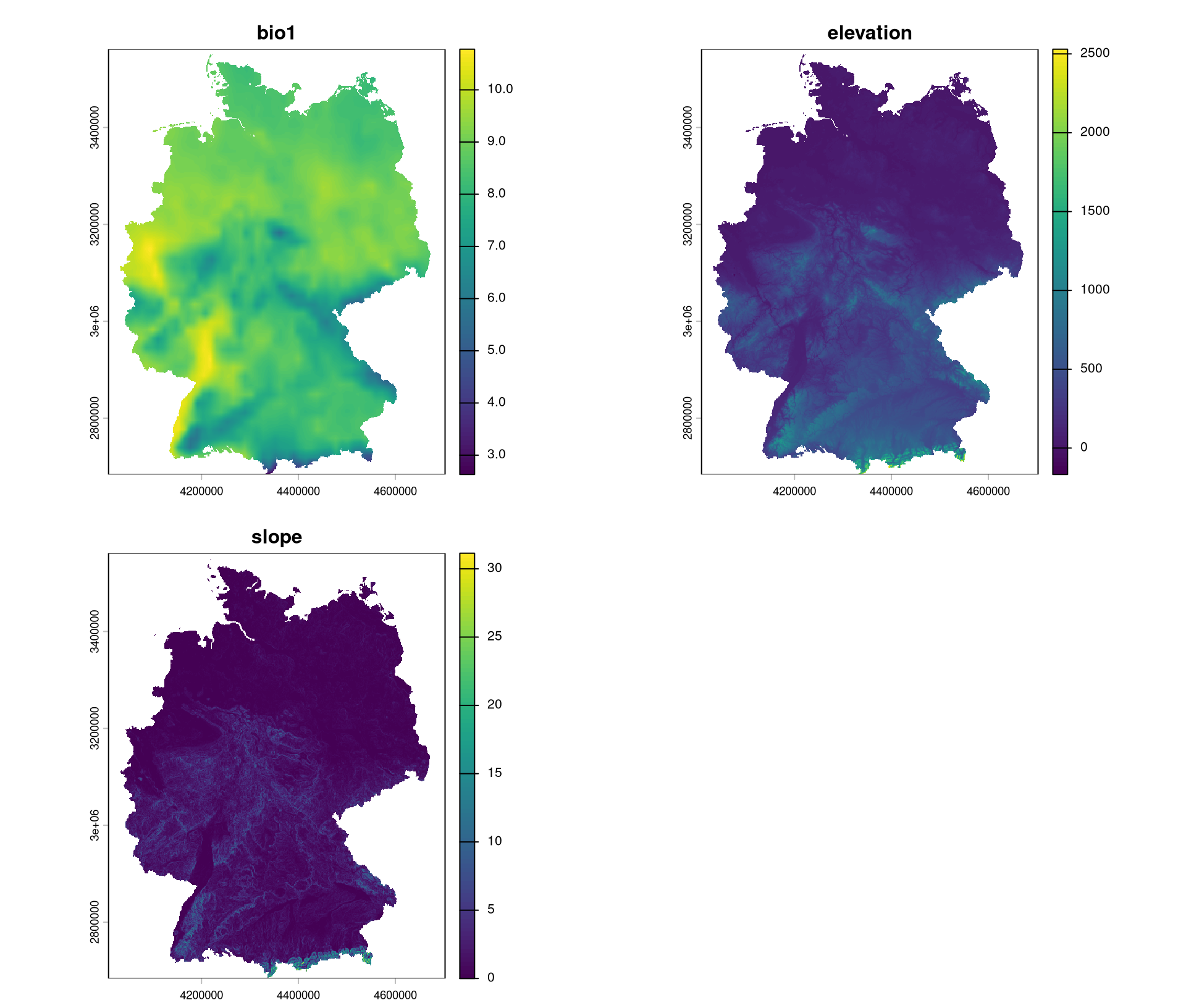
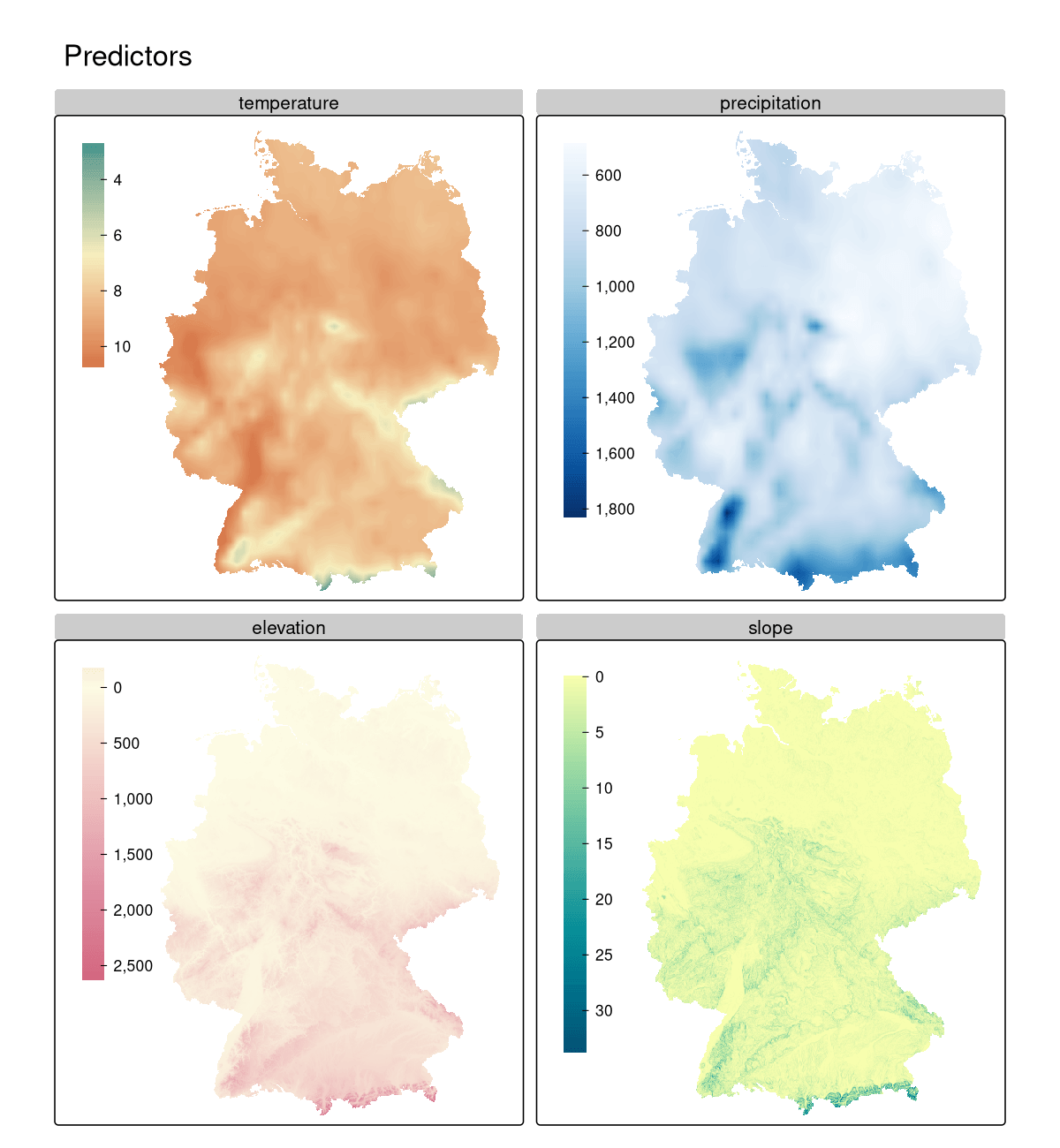
plot(predictors)

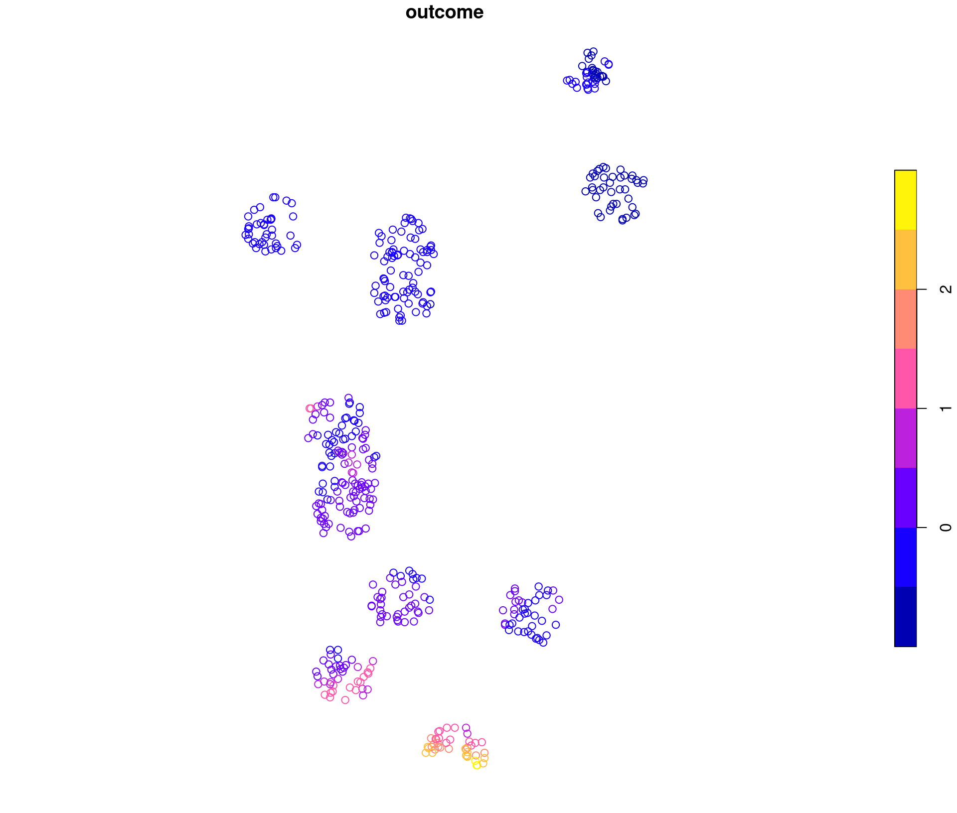
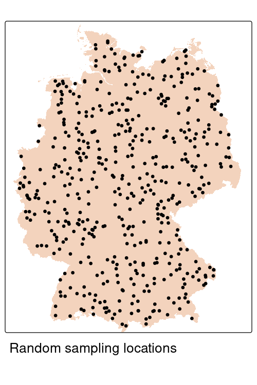
plot(samples)

Examples

Extract predictor values for the sample points and prepare training data:

samples_df <- terra::extract(predictors, 
                    samples, ID = FALSE)
samples_df <- cbind(samples, samples_df)
train_data <- samples_df |> 
  st_drop_geometry() |>
  dplyr::select(all_of(predictor_names))


Calculate the Area of Applicability (AoA) for the sample points:

aoa_data <- CAST::aoa(
  newdata = predictors,
  train = train_data,
  variables = predictor_names,
  verbose = FALSE
)
plot(aoa_data)

Examples

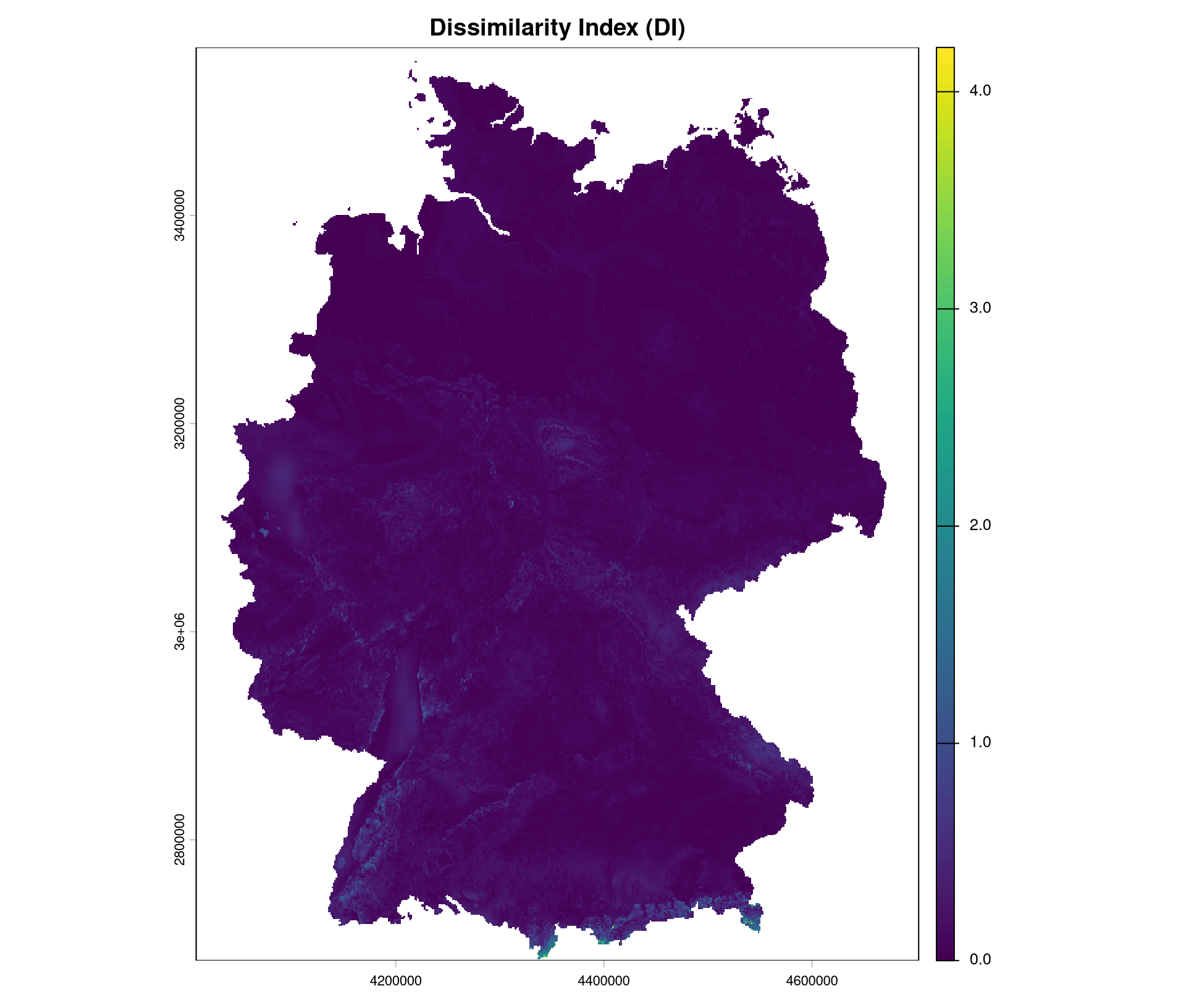
plot(aoa_data$DI, main = "Dissimilarity Index (DI)")
plot(aoa_data$AOA, main = "Area of Applicability (AOA)")
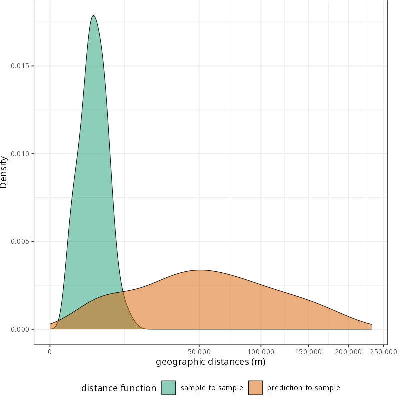
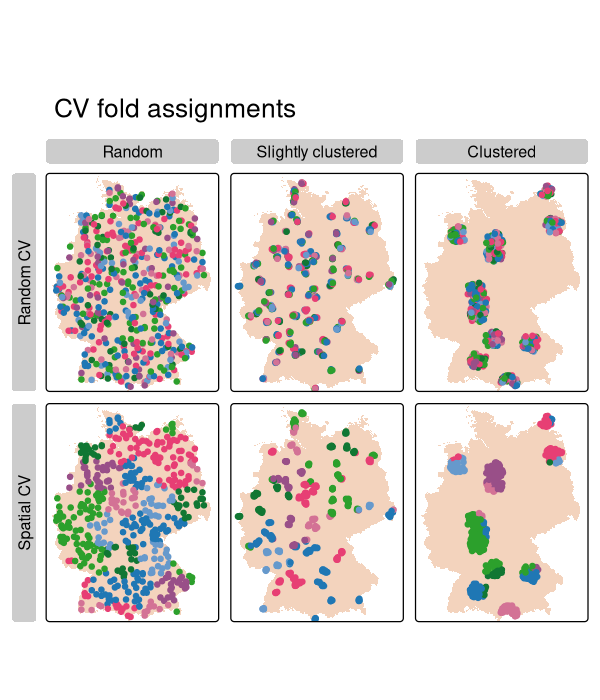
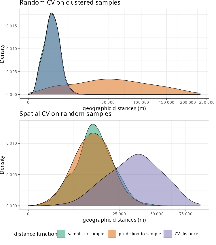
The validation strategy should follow the prediction task

Prediction difficulty depends on prediction domain

Prediction difficulty depends on prediction domain

Extrapolation continuum

Specific evaluation strategy

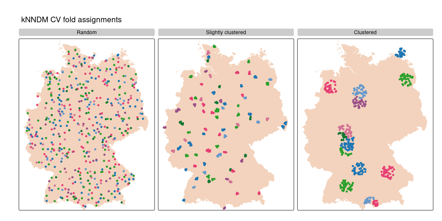
Adaptive evaluation (kNNDM)

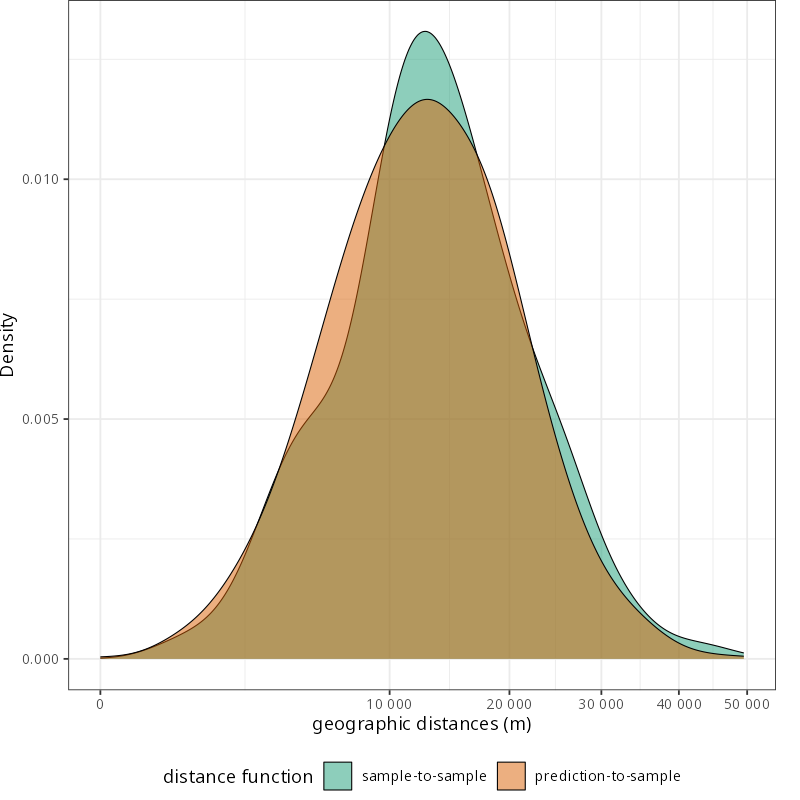
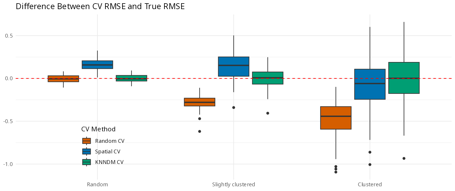
k-Nearest Neighbor Distance Matching (kNNDM, Linnenbrink et al., 2024) matches folds to the prediction scenario using distance structure (either in geographic or predictor space).
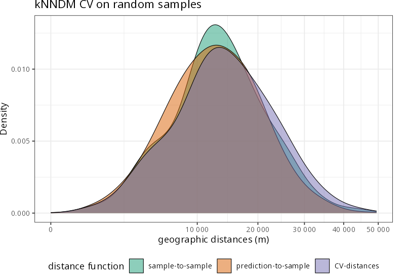
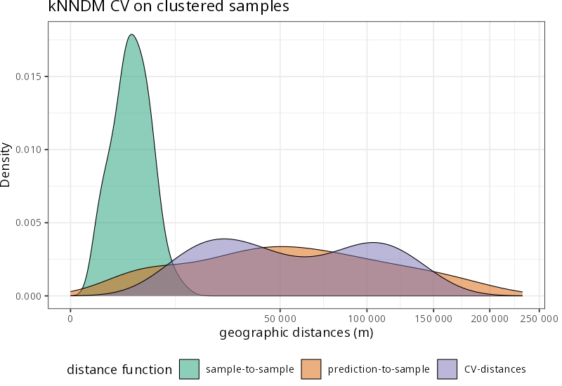
Evaluation results for different validation strategies
Examples

Create a baseline random forest model:

grid <- expand.grid(
  mtry = 2,
  splitrule = "variance",
  min.node.size = 5
)
rf_base <- train(
  x = train_data,
  y = samples_df[[response]],
  method = "ranger",
  trControl = trainControl(method = "none"),
  tuneGrid = grid,
  metric = "RMSE",
  num.trees = 300,
  importance = "impurity"
)
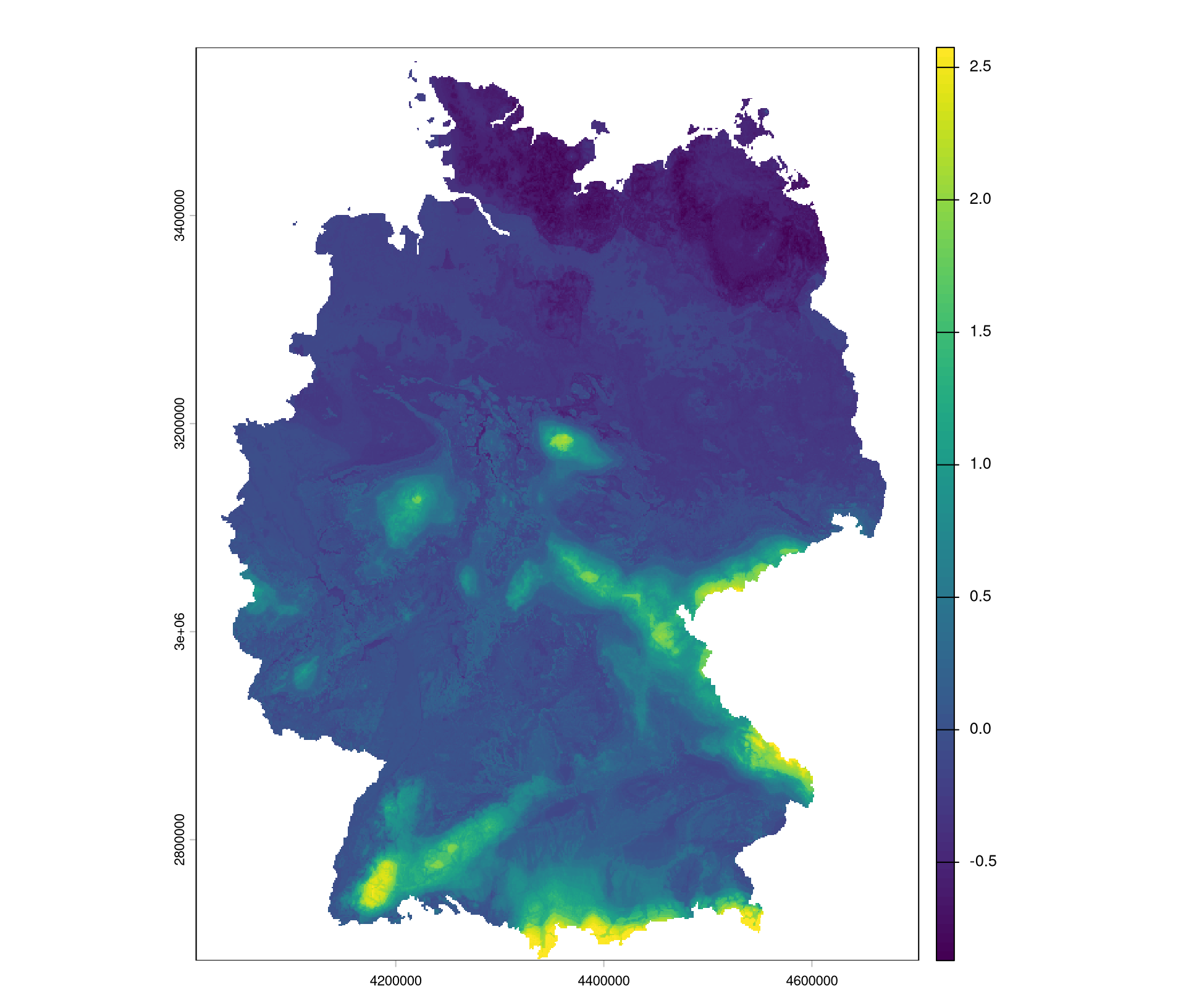
rf_base_pred <- predict(predictors, model = rf_base,
                        na.rm = TRUE)
plot(rf_base_pred)
Examples

Create a random cross-validation strategy:

random_folds <- createFolds(samples_df[[response]],
                            k = 5, 
                            returnTrain = TRUE)

indexOut <- lapply(random_folds, function(train_idx) 
                   setdiff(seq_len(nrow(samples_df)),
                   train_idx))

ctrl_random <- trainControl(
  method = "cv",
  index = random_folds,
  indexOut = indexOut,
  savePredictions = "final"
)
geodist_sr <- CAST::geodist(samples, predictors, 
                           CVtest = ctrl_random$indexOut)
plot(geodist_sr)
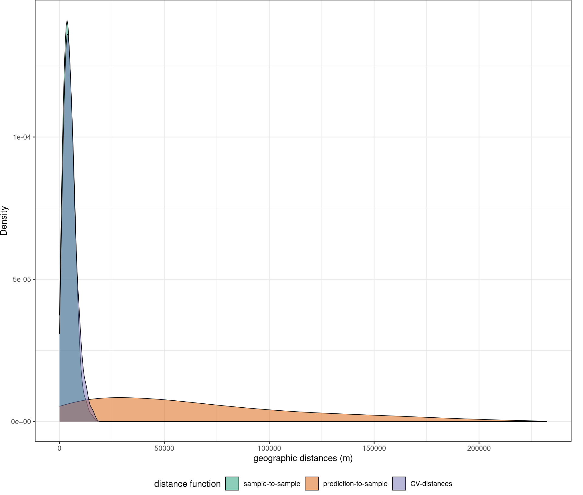
Examples

Create a kNNDM cross-validation strategy:

kn <- CAST::knndm(
  tpoints = samples_df,
  modeldomain = predictors[[1]],
  k = 5
)

ctrl_knndm <- trainControl(
  method = "cv",
  index = kn$indx_train,
  indexOut = kn$indx_test,
  savePredictions = "final",
  verboseIter = FALSE
)
geodist_sk <- CAST::geodist(samples, predictors,
                          CVtest = ctrl_knndm$indexOut)
plot(geodist_sk)
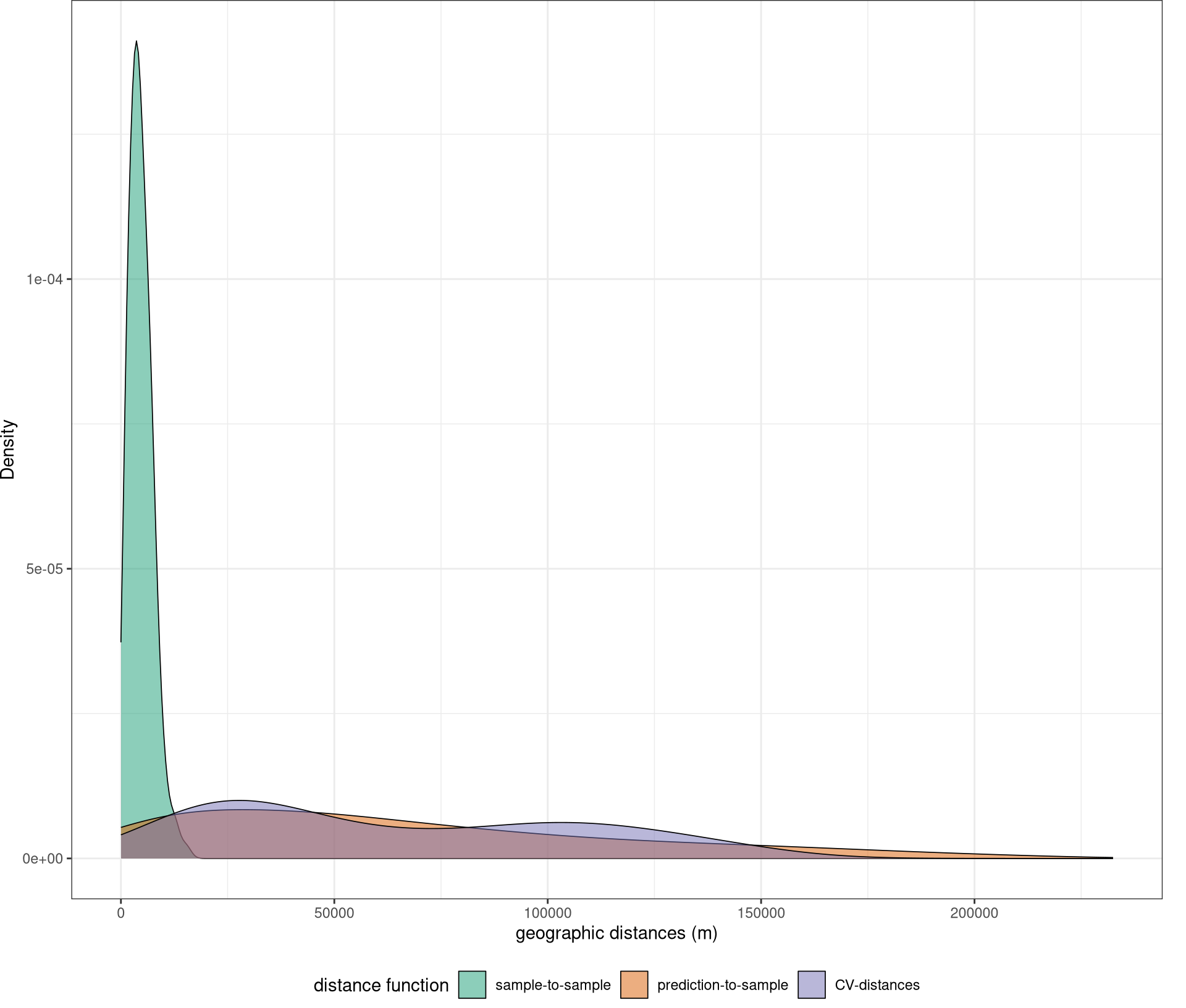
Examples

calc_rmse <- function(pred, obs){
  sqrt(mean((pred - obs) ^ 2, na.rm = TRUE))
}

Compare the RMSE of the random and kNNDM cross-validation strategies

Random cross-validation:

rf_random <- train(
  x = train_data,
  y = samples_df[[response]],
  method = "ranger",
  trControl = ctrl_random,
  tuneGrid = grid,
  metric = "RMSE",
  num.trees = 300,
  importance = "impurity"
)
random_rmse <- calc_rmse(rf_random$pred$pred,
                         rf_random$pred$obs)
random_rmse
[1] 0.145039

kNNDM cross-validation:

rf_knndm <- train(
  x = train_data,
  y = samples_df[[response]],
  method = "ranger",
  trControl = ctrl_knndm,
  tuneGrid = grid,
  metric = "RMSE",
  num.trees = 300,
  importance = "impurity"
)
knndm_rmse <- calc_rmse(rf_knndm$pred$pred,
                        rf_knndm$pred$obs)
knndm_rmse
[1] 0.2379049

Examples

Given that this is a simulation study, we can also compare the RMSE of the cross-validation strategies to the true RMSE of the model predictions across the whole area of interest.

true_outcome_raster <- rast("data/germany/true_outcome/true_outcome.tif")
rf_base_pred_values <- terra::values(rf_base_pred, mat = FALSE)
true_outcome_raster_values <- terra::values(true_outcome_raster, mat = FALSE)
true_rmse <- calc_rmse(rf_base_pred_values, true_outcome_raster_values)


Comparison of RMSE values for the random CV, kNNDM CV, and true RMSE:

rmse_results <- data.frame(
  Method = c("Random CV", "kNNDM CV", "True RMSE"),
  RMSE = c(random_rmse, knndm_rmse, true_rmse)
)
rmse_results
     Method      RMSE
1 Random CV 0.1450390
2  kNNDM CV 0.2379049
3 True RMSE 0.2682184

Examples

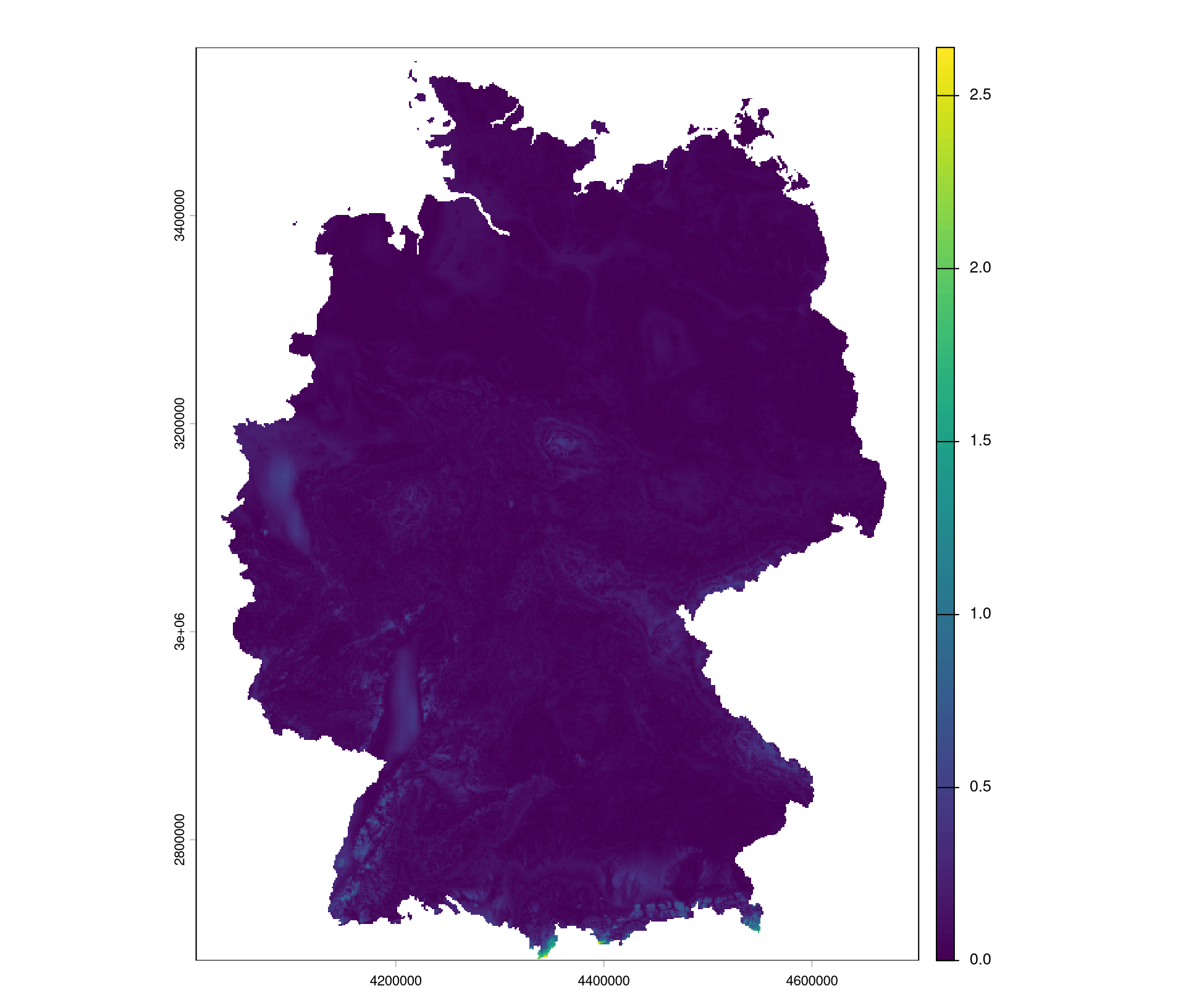
Apply the Area of Applicability (AoA) analysis to the kNNDM model predictions:

aoa_model_knndm <- aoa(newdata = predictors, model = rf_knndm, verbose = FALSE)
plot(aoa_model_knndm)

plot(aoa_model_knndm$DI)
plot(aoa_model_knndm$AOA)
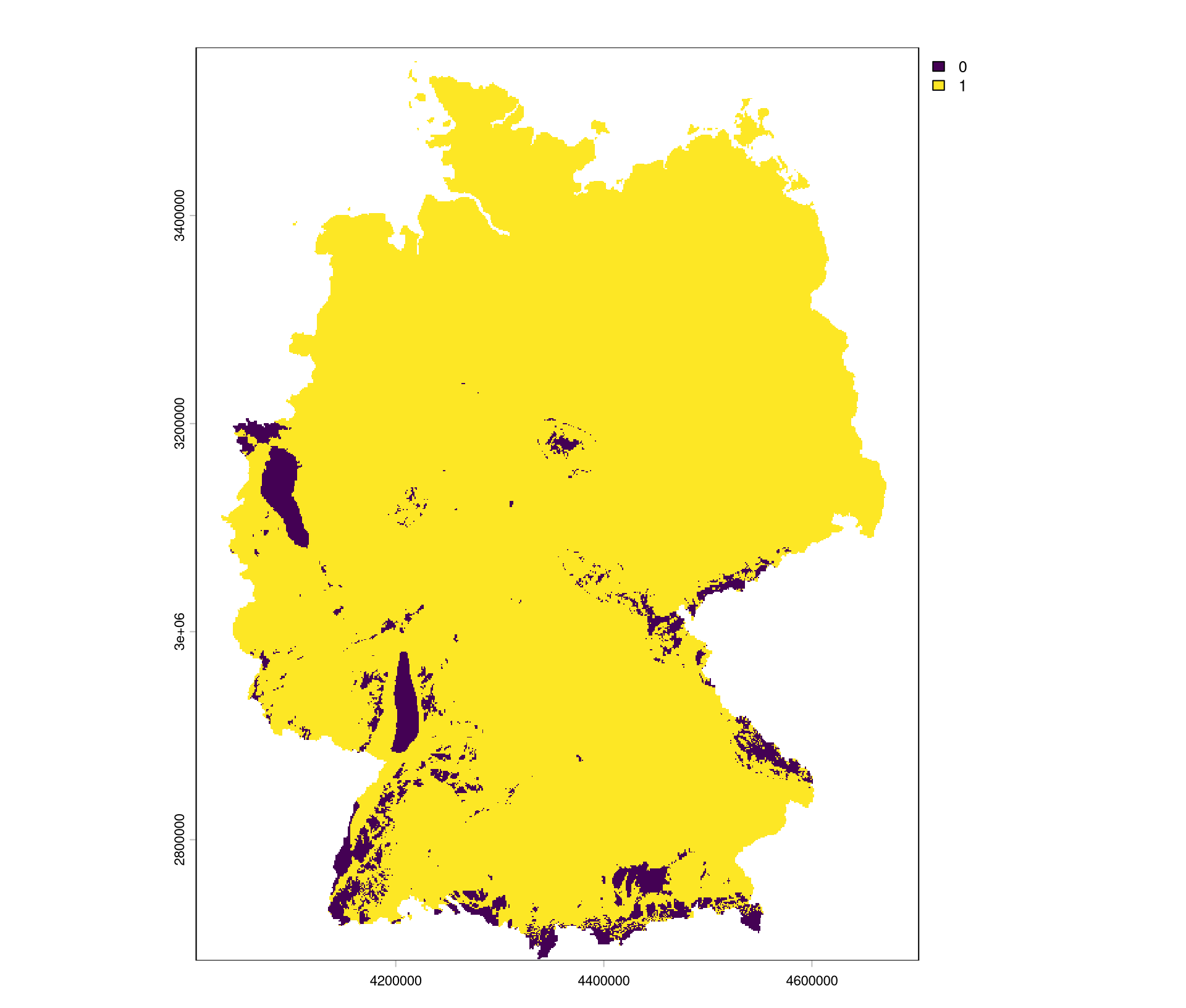
Error profiles

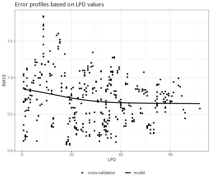
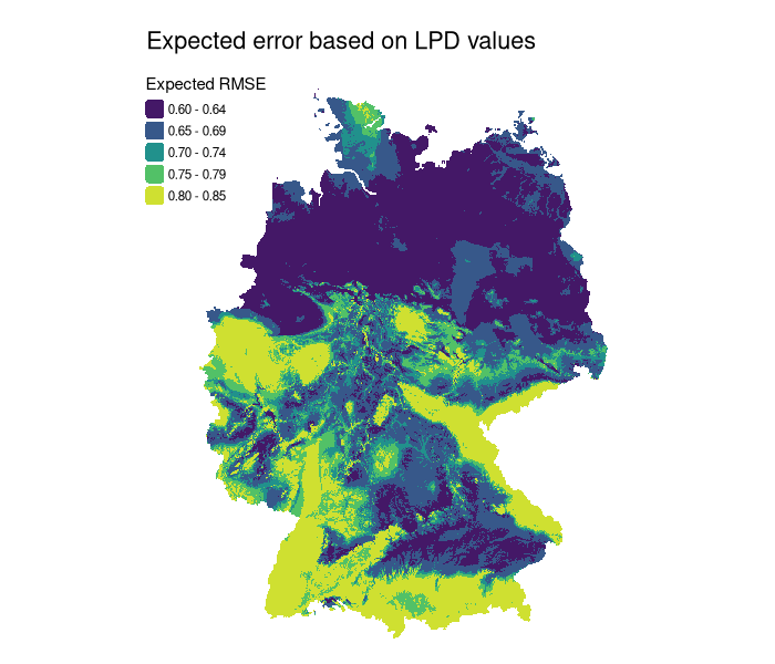
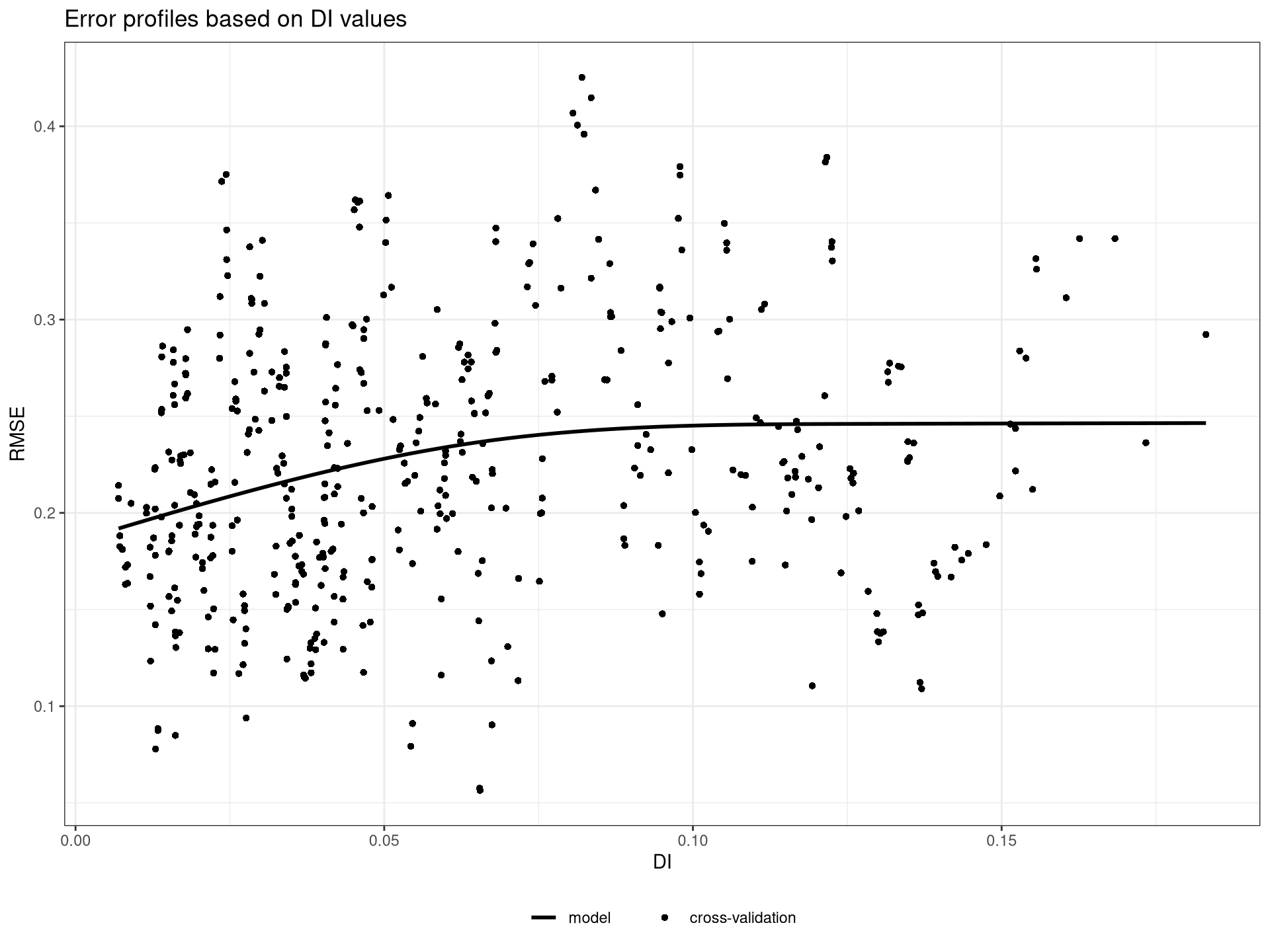
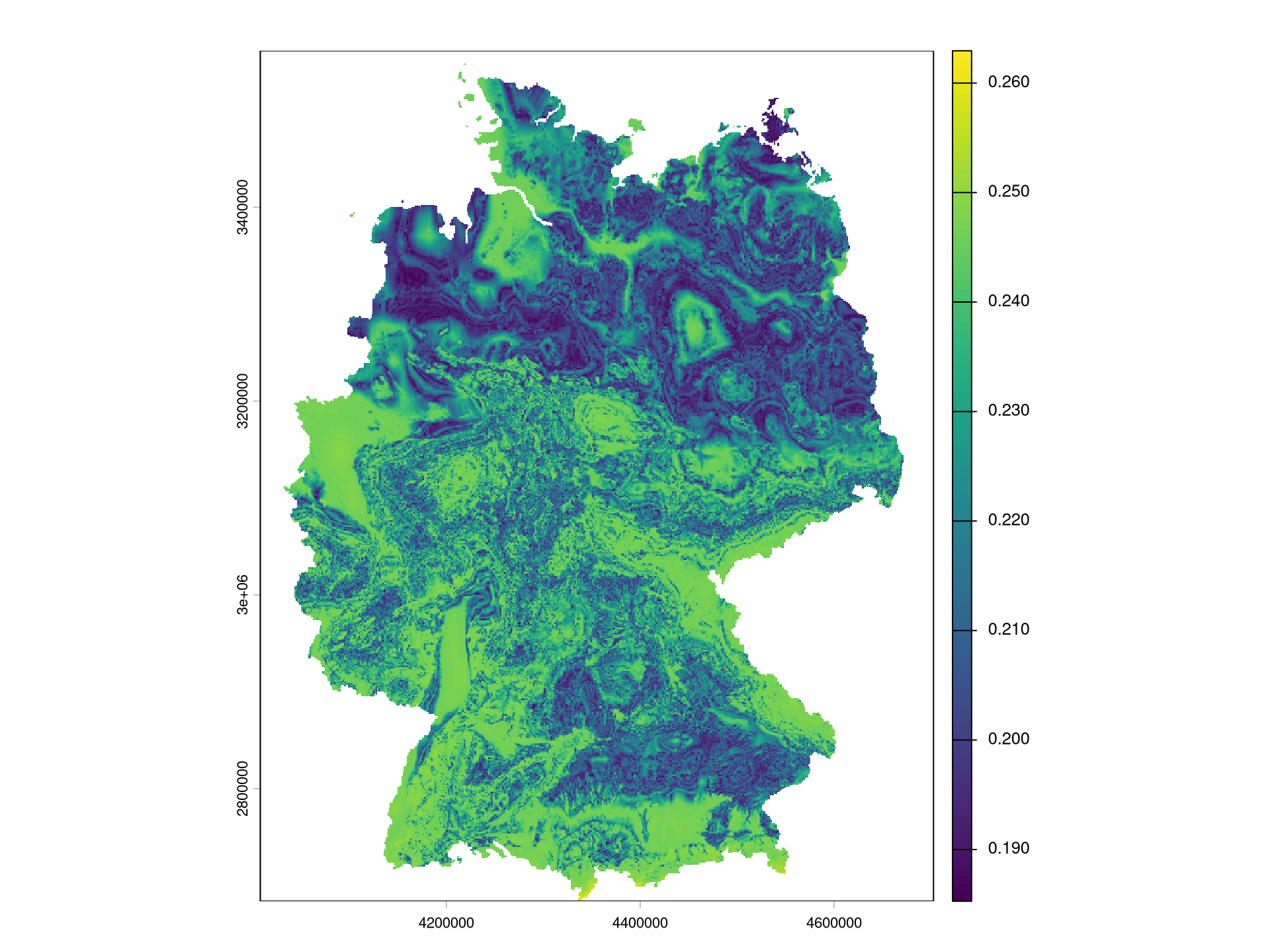
Error profiles show how expected error (based on DI or LPD) relates to true error. They can be used to identify where predictions are more or less trustworthy, and to adjust the AoA threshold or interpret LPD values.
Examples

errormodel <- errorProfiles(rf_knndm, aoa_model_knndm, 
                            variable = "DI")
plot(errormodel) +
  ggtitle("Error profiles based on DI values")
expected_error_DI <- terra::predict(aoa_model_knndm$DI, 
                                    errormodel)
plot(expected_error_DI)
Prediction conditions are not equally common

Overlapping predictor distribution(s)

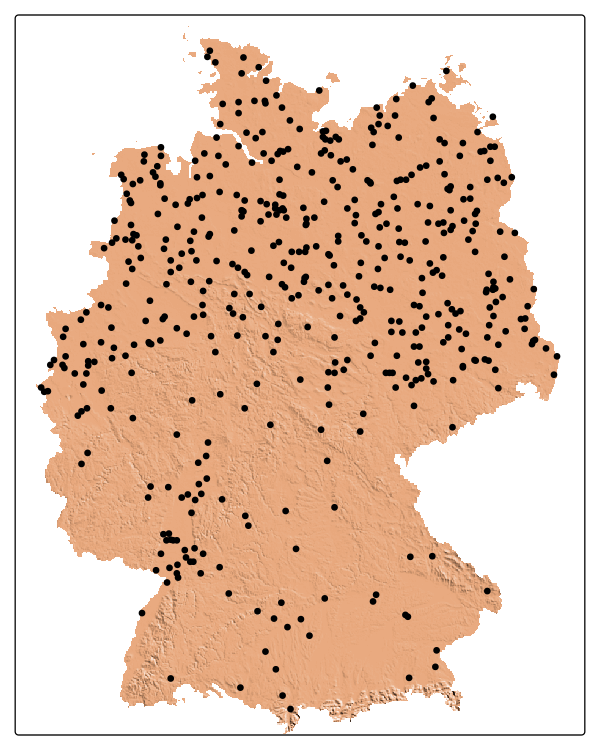
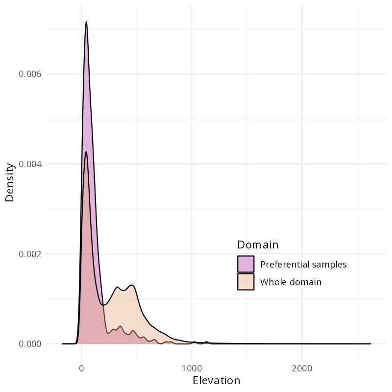
Partially overlapping predictor distribution(s)

Weighting validation points

Evaluation approach Lowland-area weight (%) Highland-area weight (%) Overall RMSE
Germany domain (target distribution) 50 50 0.667
Preferential sample (unweighted) 89 11 0.541
Preferential sample (reweighted) 50 50 0.667

Approaches to reweighting

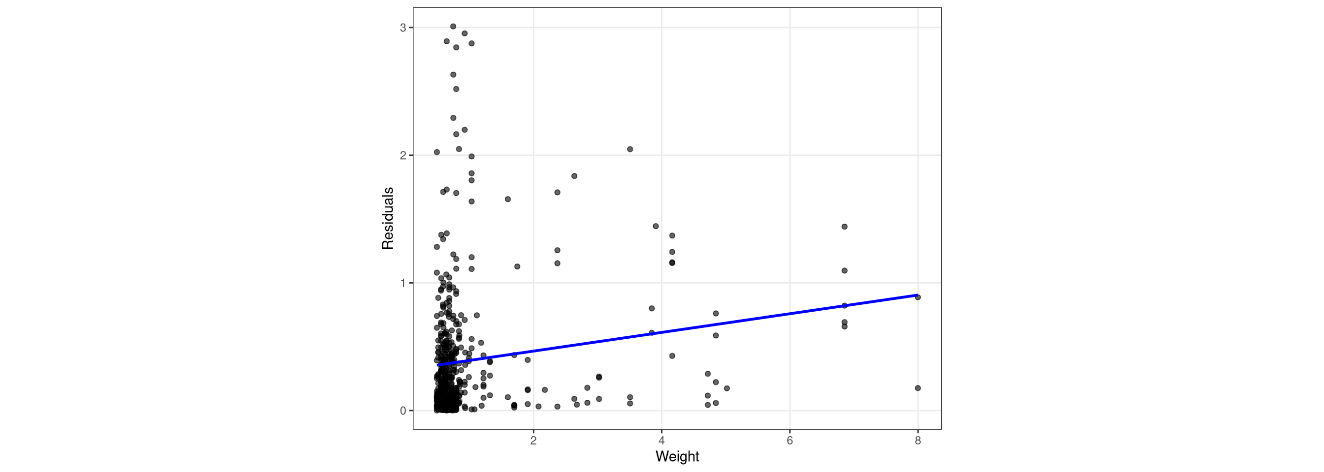
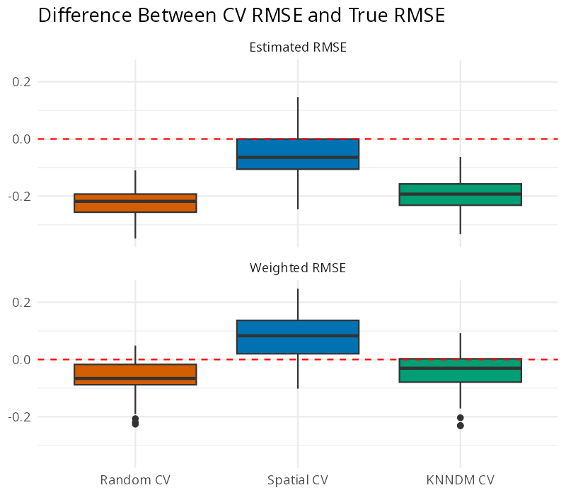
Target-Weighted Cross-Validation (TWCV, Brenning and Suesse, 2026) adjusts cross-validation weights to align evaluation with the prediction domain rather than the sampled data distribution.
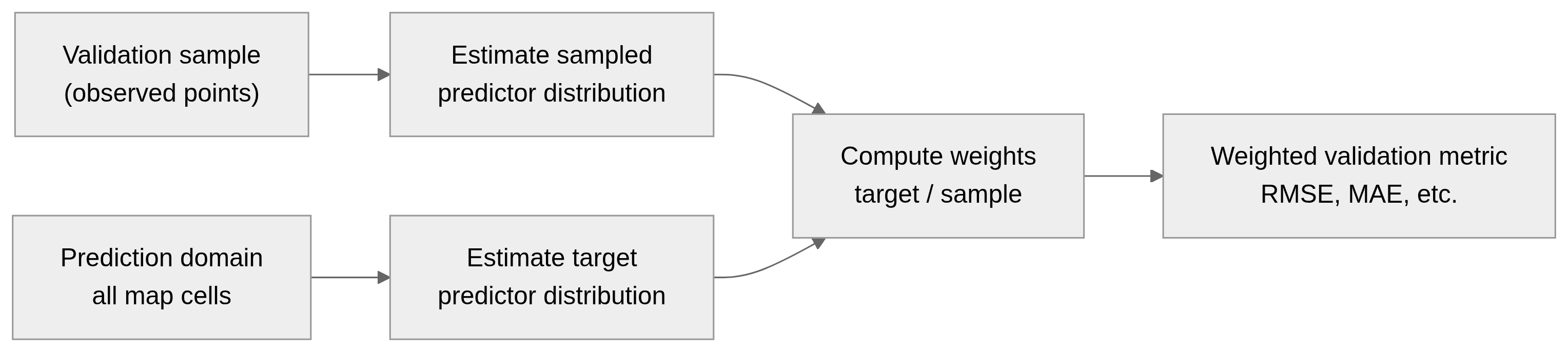

Effect of weighting validation points
Examples

This time we have a preferential sample.

pref_samples <- 
  read_sf("data/germany/samples/pref_samples.gpkg")
pref_samples_df <- terra::extract(predictors, 
                    pref_samples, ID = FALSE)
pref_samples_df <- cbind(pref_samples, pref_samples_df)
pref_train_data <- pref_samples_df |> 
  st_drop_geometry() |>
  dplyr::select(all_of(predictor_names))
grid <- expand.grid(
  mtry = 2,
  splitrule = "variance",
  min.node.size = 5
)
pref_rf_base <- train(
  x = pref_train_data,
  y = pref_samples_df[[response]],
  method = "ranger",
  trControl = trainControl(method = "none"),
  tuneGrid = grid,
  metric = "RMSE",
  num.trees = 300,
  importance = "impurity"
)

Examples

pref_rf_base_pred <- predict(predictors, 
                             model = pref_rf_base,
                             na.rm = TRUE)
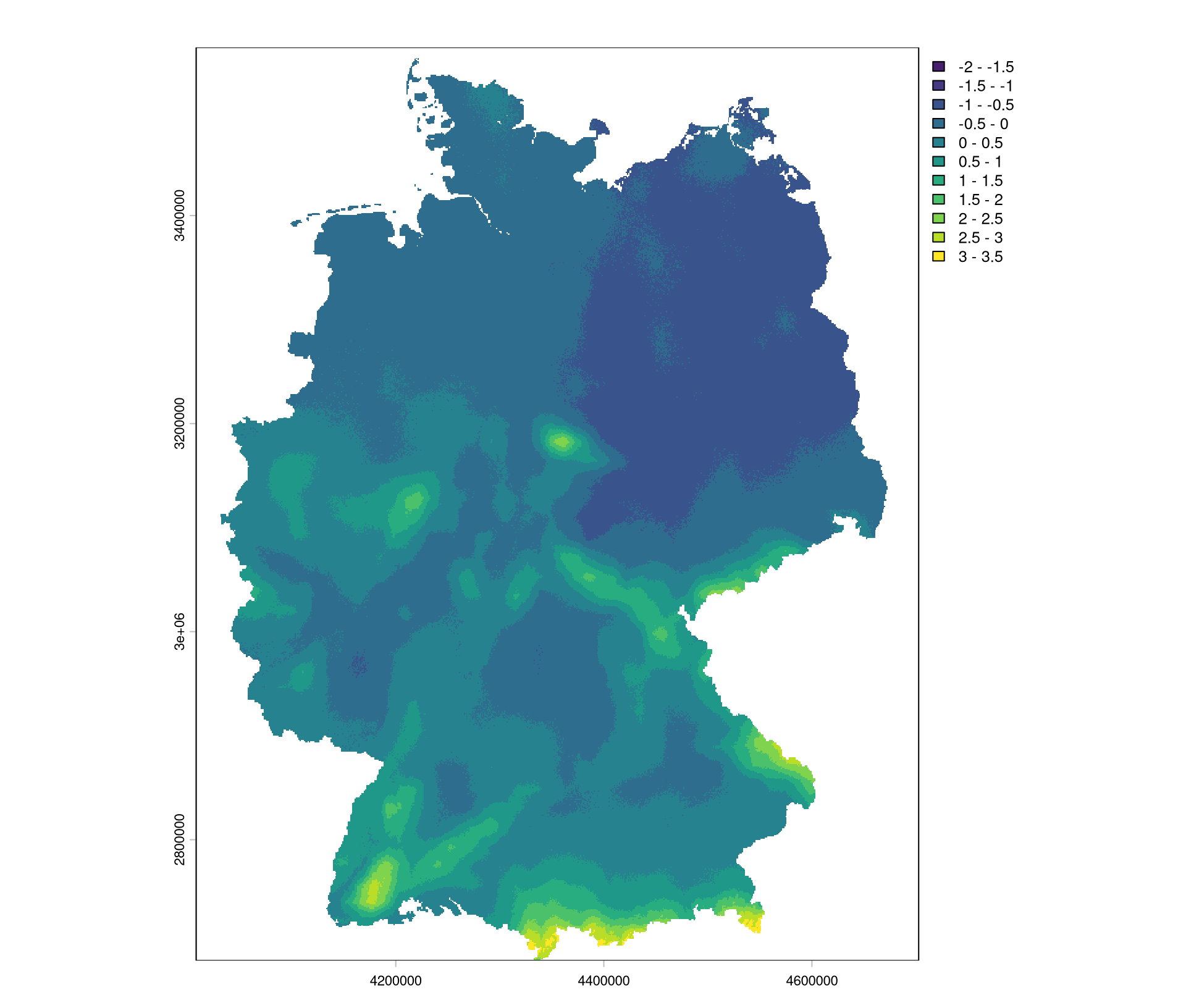
plot(pref_rf_base_pred, breaks = seq(-2, 3.5, 0.5))
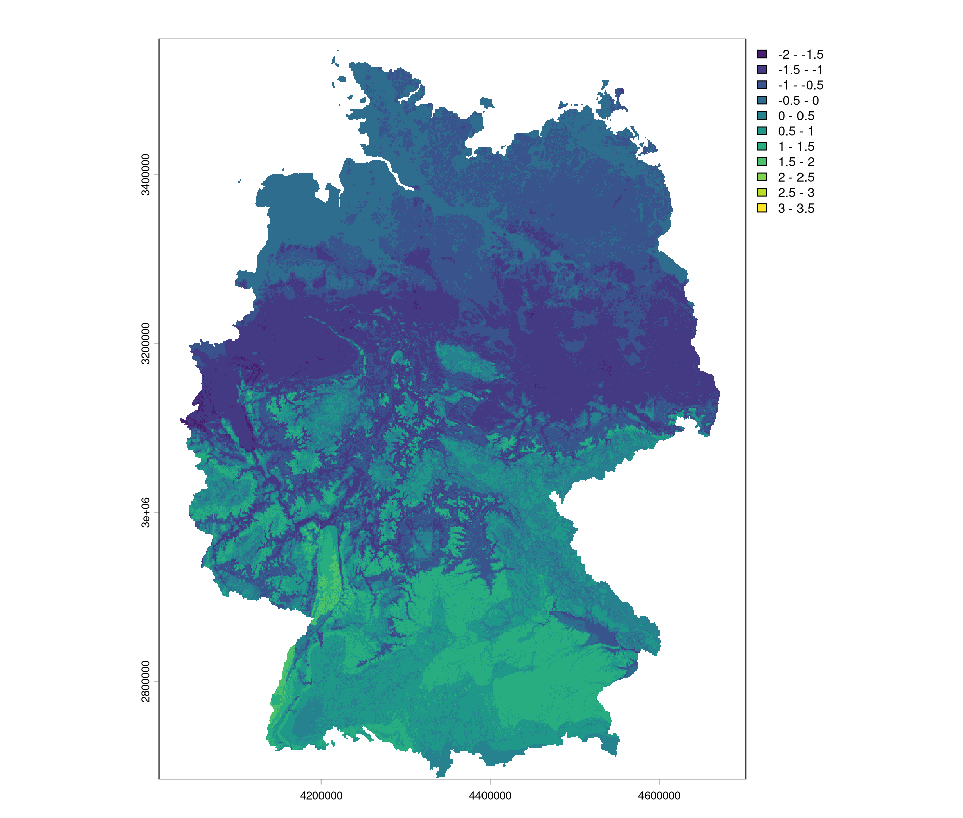
rast("data/germany/true_outcome/true_outcome.tif") |>
  plot(breaks = seq(-2, 3.5, 0.5))
Examples

kn <- CAST::knndm(tpoints = pref_samples_df,
                  modeldomain = predictors[[1]],  k = 5)

ctrl_knndm <- trainControl(
  method = "cv",  index = kn$indx_train,
  indexOut = kn$indx_test, savePredictions = "final",
  verboseIter = FALSE
)

pref_rf_knndm <- train(
  x = pref_train_data, y = pref_samples_df[[response]],
  method = "ranger", trControl = ctrl_knndm,
  tuneGrid = grid, metric = "RMSE",
  num.trees = 300, importance = "impurity"
)
pref_knndm_rmse <- calc_rmse(pref_rf_knndm$pred$pred,
                             pref_rf_knndm$pred$obs)
pref_knndm_rmse
[1] 0.6411687
pref_rf_base_pred_values <- 
  terra::values(pref_rf_base_pred, mat = FALSE)
true_outcome_raster_values <- 
  terra::values(true_outcome_raster, mat = FALSE)
pref_true_rmse <- 
  calc_rmse(pref_rf_base_pred_values,
            true_outcome_raster_values)
pref_true_rmse
[1] 0.781608

Examples

The PredictionMatching package is still under heavy development, and the API may change in the future. Please check the PredictionMatching GitHub repository

library(PredictionMatching) # pak::pak("JanLinnenbrink/PredictionMatching")
w <- tw_calculate_weights(tpoints = pref_train_data, modeldomain = predictors)
pe <- tw_pointwise_error(obs = pref_rf_knndm$pred$obs, pred = pref_rf_knndm$pred$pred, 
                         id = pref_rf_knndm$pred$rowIndex)
plot(w, pointwise_error = pe)[[2]]

Examples

weighted_rmse <- tw_weighted_error_stats(w, pe)[["rmse"]]
weighted_rmse
[1] 0.7209784


RMSE
True RMSE 0.782
KNN-DM RMSE 0.641
Weighted RMSE 0.721

Prediction-domain adaptive evaluation

Prediction-domain adaptive evaluation

Key components:

  1. Define the prediction domain
  2. Construct validation folds that reflect the prediction domain
  3. Weight validation samples by their prevalence in the prediction domain


Open questions remain, including how to mix these three components together (e.g., how to weight folds, should we define the prediction domain in advance before constructing folds, etc.).

Summary

  • For predictive spatial machine learning, we should evaluate the map, not the model
  • Evaluation should reflect the prediction scenario, not just the sample at hand
  • Three approaches can help to achieve this:
    1. define the prediction domain,
    2. construct validation folds that reflect the prediction domain
    3. weight validation samples by their prevalence in the prediction domain
  • Tools to use these approaches are available
  • Prediction-domain adaptive evaluation solves some problems, but not all problems (e.g., uncertainty quantification, spatial autocorrelation in residuals, metric selection, temporal transfer, scale mismatch, explainability, etc.)
Contact

https://jakubnowosad.com

Resources

Our current related work: Nowosad et al., 2026, Linnenbrink et al., 2026

Slides:

Acknowledgements