Create a Patternogram or a Patternogram Cloud — patternogram • patternogram

It creates a patternogram or a patternogram cloud. The function takes a raster object of class SpatRaster or a point vector object of class sf as input, and calculates the dissimilarity between values of pairs of points given the distances between them. The output of this function is a tibble of the patternogram class that can be visualized with the plot() and autoplot() functions.

patternogram(
  x,
  cutoff,
  width = cutoff/15,
  dist_fun = "euclidean",
  sample_size = 100,
  cloud = FALSE,
  target = NULL,
  ...
)

Arguments

x: A raster object of class SpatRaster (terra) or a point vector object of class sf (sf)
cutoff: Spatial distance up to which point pairs are included in patternogram estimates; by default: a square root of the raster area
width: The width of subsequent distance intervals for which data point pairs are grouped for patternogram estimates
dist_fun: Distance measure used. This function uses the philentropy::distance() function (run philentropy::getDistMethods() to find possible distance measures)
sample_size: Only used when x is raster. Proportion of the cells inside of each region to be used in calculations. Value between 0 and 1. It is also possible to specify an integer larger than 1, in which case the specified number of cells of each region will be used in calculations.
cloud: Logical; if TRUE, calculate the patternogram cloud
target: Additional argument allowing to calculate separate estimates for different categories or ranges of values
...: Additional arguments for base::cut()

Value

A tibble of the patternogram class with columns, such as (a) np - the number of point pairs in this estimate, (b) dist - the middle of the distance interval used for each estimate, (c) dissimilarity - the dissimilarity estimate, (d) (optional) target

Examples

r = terra::rast(system.file("ex/elev.tif", package = "terra"))
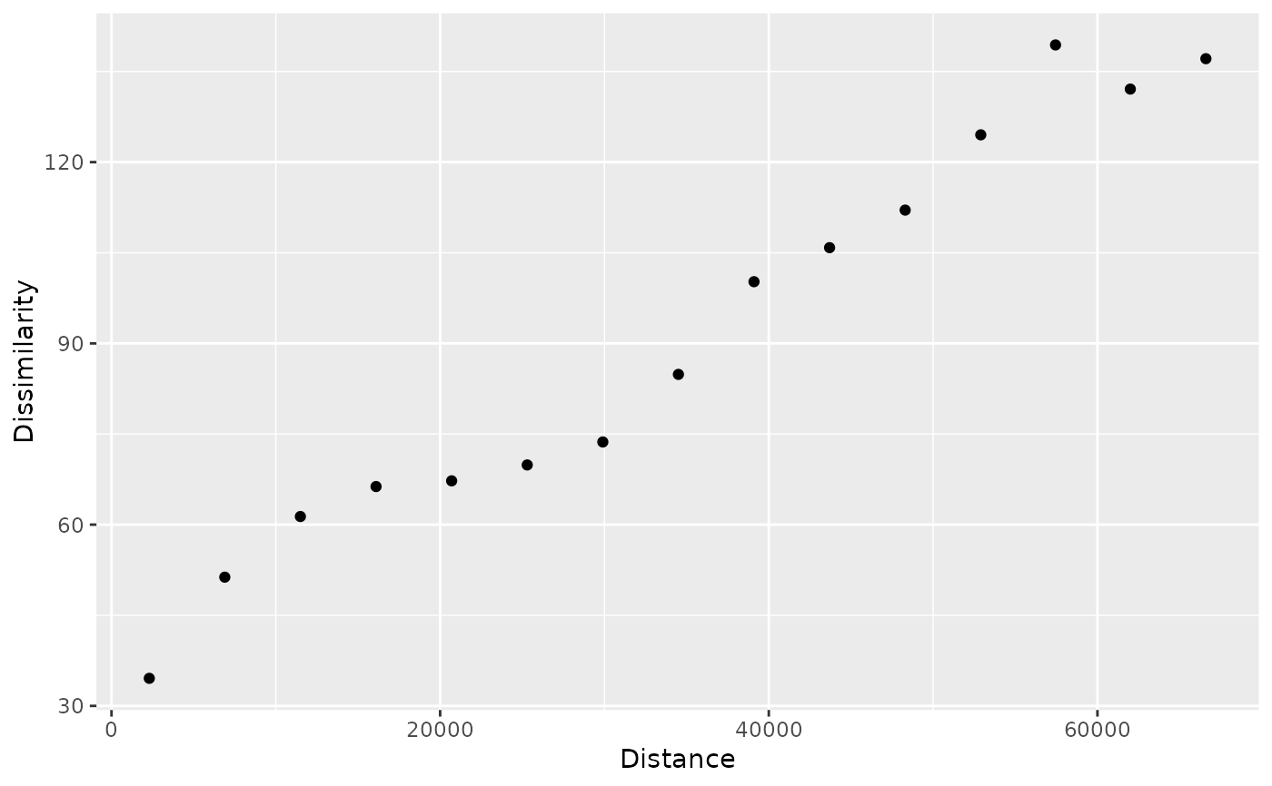
pr = patternogram(r)
pr
#> # A tibble: 15 × 3
#>       np  dist dissimilarity
#>  * <int> <dbl>         <dbl>
#>  1   129  2300          34.6
#>  2   326  6895          51.3
#>  3   459 11495          61.3
#>  4   554 16100          66.3
#>  5   541 20700          67.3
#>  6   530 25300          69.9
#>  7   495 29900          73.7
#>  8   501 34500          84.9
#>  9   414 39100         100. 
#> 10   294 43700         106. 
#> 11   237 48300         112. 
#> 12   181 52900         125. 
#> 13   123 57450         139. 
#> 14    88 62000         132. 
#> 15    41 66600         137. 
plot(pr)