Making maps of the USA with R: alternative layout

Update (2018-12-12): Alternative approach to this problem can be found at https://github.com/Nowosad/us-map-alternative-layout.

Introduction

Maps of United States often focus only on the contiguous 48 states. In many maps Alaska and Hawaii are simply not shown or are displayed at different geographic scales than the main map. This article shows how to create inset maps of the USA, building on a chapter in the in-development book Geocomputation with R that shows all its states and ensures relative sizes are preserved.

It requires up-to-date versions of the following packages to be loaded:¹

# devtools::install_github("robinlovelace/geocompr") # install pkgs
library(spData) # contains datasets used in this example
library(sf)     # for handling spatial (vector) data
library(tmap)   # map making package
library(grid)   # to re-arrange maps

Data preparation

First, we must decide on the best projection for each inset. For this case, we will use equal area projection. Hawaii and Alaska already come with an appropriate projection (US National Atlas Equal Area) but us_states (provided by spData) must be reprojected:

us_states2163 = st_transform(us_states, 2163)

Ratio calculation

The next step is to calculate scale relations between the mainland and Hawaii as well as Alaska. To do so we can calculate latitude ranges of the bounding box of each object:

us_states_range = st_bbox(us_states2163)[4] - st_bbox(us_states2163)[2]
hawaii_range = st_bbox(hawaii)[4] - st_bbox(hawaii)[2]
alaska_range = st_bbox(alaska)[4] - st_bbox(alaska)[2]

Next, we can calculate the ratios between their areas:

us_states_hawaii_ratio = hawaii_range / us_states_range
us_states_alaska_ratio = alaska_range / us_states_range

Map and inset map creation

In the third step, we need to create single maps for each object. The tm_layout() function is used here to remove map frames and backgrounds or to add titles to our insets:

us_states_map = tm_shape(us_states2163) +
  tm_polygons() + 
  tm_layout(frame = FALSE)

hawaii_map = tm_shape(hawaii) +
  tm_polygons() + 
  tm_layout(title = "Hawaii", frame = FALSE, bg.color = NA, 
            title.position = c("LEFT", "BOTTOM")) 

alaska_map = tm_shape(alaska) +
  tm_polygons() + 
  tm_layout(title = "Alaska", frame = FALSE, bg.color = NA, 
            title.position = c("left", "TOP")) 

Map arrangement

The final step is to arrange the map, using the grid package. The code below creates a new ‘page’ and specifies its layout with two rows - one smaller (for Alaska) and one larger (for the contiguous 48 states). Each inset map is printed in its corresponding viewport, with Hawaii is printed in the bottom of the second row. Note the use of ratios to make the size of Alaska and Hawaii roughly comparable with that of the main land. The final step draws dashed lines (gp = gpar(lty = 2)) to separate mainland from Alaska and Hawaii.

grid.newpage()
pushViewport(viewport(layout = grid.layout(2, 1,
                                           heights = unit(c(us_states_alaska_ratio, 1), "null"))))
print(alaska_map, vp = viewport(layout.pos.row = 1))
print(us_states_map, vp = viewport(layout.pos.row = 2))
print(hawaii_map, vp = viewport(x = 0.3, y = 0.07,
                                height = us_states_hawaii_ratio / sum(c(us_states_alaska_ratio, 1))))
grid.lines(x = c(0, 1), y = c(0.58, 0.58), gp = gpar(lty = 2))
grid.lines(x = c(0, 0.5), y = c(0.33, 0), gp = gpar(lty = 2))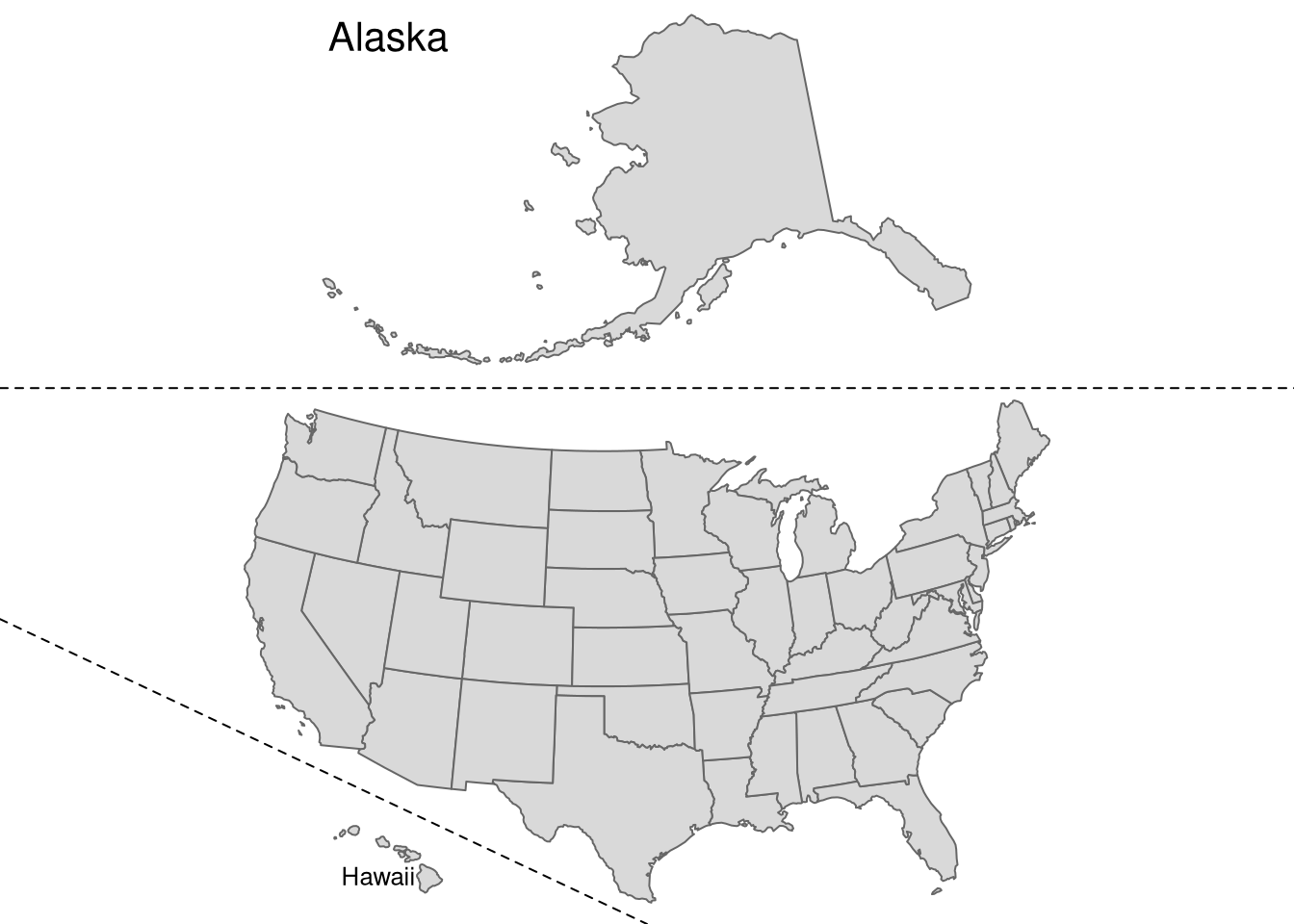

Final words

The final map is an approximation of areal relationships between the mainland, Alaska and Hawaii. This improves on maps of the United States that only show the mainland or greatly reduce the relative size of Hawaii and Alaska.

But there is scope for further improvement building on the reproducible code above (a fun challenge is to recreate the map without any copy-pasting): I look forward to any suggestions how this map can be improved! Contact me on twitter or github - see information below.

The blogpost builds on the content in Chapter 8 of the book Geocomputation with R. A regularly updated online version of the Geocomputation with R book can be found at https://geocompr.robinlovelace.net/. It can be edited from our github repo or by clicking on the ‘edit’ pencil-shaped symbol at the top left of any part of the book:

I also encourage community contributions on any part of the book, for example by using the issue tracker.

Footnotes

1. These packages can be installed individually with install.packages("spData") etc or by uncommenting and executing the first command in the code chunk, which installs all packages needed to reproduce the code in Geocomputation with R.