sabre: or how to compare two maps?

Creating or determination of regions is a useful way to describe the world. Regionalization does not only allow for a quicker understanding of spatial patterns but also can influence how regions are managed. Regions are created in various disciplines. We can delineate regions based on a single property (e.g. landform regions or climate regions) or several factors (e.g. ecoregions). There are also political regions divided by borders that are established through political or social agreements. Regions are powerful also because they can be easily visualized.

On the other hand, it is difficult to compare different regionalizations. For example, you have two regionalizations based on the same property but from two different times and you want to know how similar they are to each other and where the largest change had occurred. Another example is when you have two maps of the same property created by two different entities and you want to know where they are in agreement and where they are very different. Comparing different regionalizations also apply when we have two maps of different properties and we want to know is there a spatial relationship between the first regionalization and the second one.

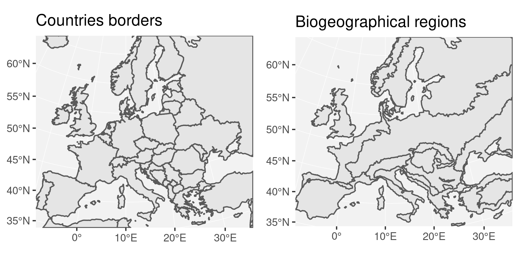
European countries map (left). Biogeographical regions of Europe (right)

The figure above is the simplest way of comparison - a visual approach by plotting two maps side by side. Now you could take a look at the map on the left, decide on some area of interest and next try to locate the same area on the map on the right side. Alternatively, it is possible to use lines to indicate the first regionalization, and color to express the second regionalization:

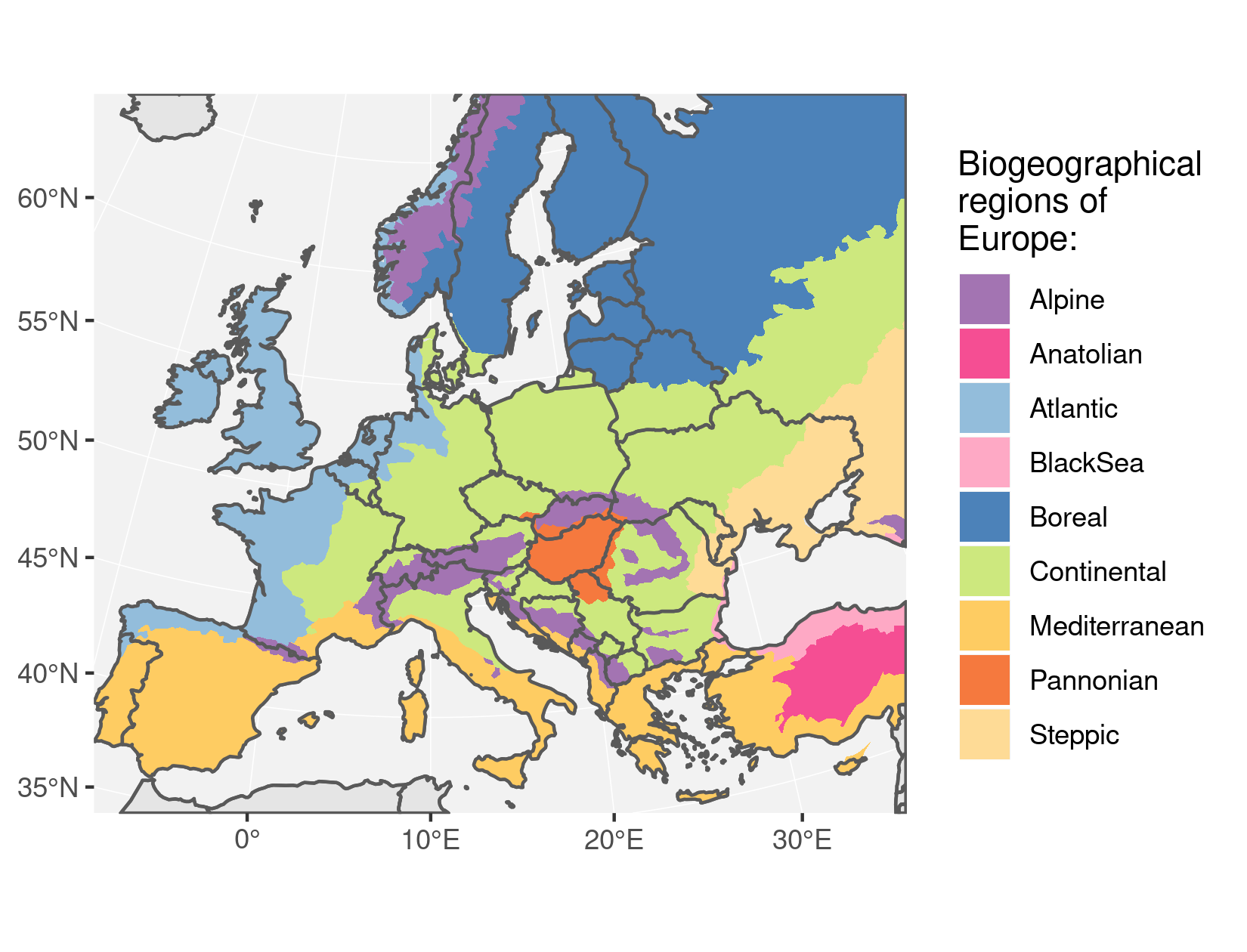
Borders of European countries superimposed on the biogeographical regions of Europe

This way it is easy to see that the Netherlands lies in only one biogeographic region “Atlantic”, while some countries are in two or more biogeographic regions. There are also several ways to compare regionalization maps interactively, for example using tmap::tmap_arrange() in the view mode or the mapview::slideView() function.

There is still one issue though - how to compare two regionalizations quantitatively? In other words - how to calculate a similarity between two regionalizations or categorical maps? For this purpose, we developed a new R package called sabre, which stands for Spatial Association Between REegionalizations. You can download it from CRAN:

install.packages("sabre")

In this blogpost, we will use only two R packages:

# attach packages
library(sf)
library(sabre)

Additionally, ggplot2 was used to create the maps and gganimate to create the animations.

Data

Let’s try this package by using the two datasets mentioned above - the first one consists of counties borders and the second one represents biogeographical regions of Europe. They could be downloaded through R with:

# data download
url = "https://github.com/Nowosad/bp-data/raw/main/2018-09-10-sabre-bp/regions.zip"
download.file(url, destfile = "regions.zip")
unzip("regions.zip", exdir = "data")

Importantly, sabre requires that two input datasets have the same coordinate reference system (CRS). If your datasets have different CRS’s, you can transform one of the datasets to have the same CRS as the second one. To learn more read the section about reprojecting vector geometries from the Geocomputation with R book.

Next, we just need to read the data:

# read data
europe_borders = st_read("data/europe_borders.gpkg", quiet = TRUE)
biogeo_regions = st_read("data/biogeo_regions.gpkg", quiet = TRUE)

Note: the sabre package expects data with valid geometries only. You can fix invalid geometries with sf::st_make_valid().

V-measure

The main function in sabre is vmeasure_calc(). It calculates a degree of spatial association between two regionalizations using an information-theoretical measure called the V-measure. We adapted this measure from computer science, where it is used to compare (non-spatial) clusterings (Rosenberg and Hirschberg, 2007).

V-measure is built upon two intermediate metrics - homogeneity and completeness. Homogeneity is a measure of how well regions from the first map fit inside of regions from the second map. Completeness measures how well regions from the second map fit inside of regions from the first map. The final value of v-measure is calculated as the weighted harmonic mean of homogeneity and completeness. All of these metrics have values between 0 and 1, where larger values indicate better spatial agreement.

Comparision between two maps

The vmeasure_calc() function requires four arguments:

• x - a name of spatial object (map 1)
• y - a name of spatial object (map 2)
• x_name - a name of the column with regions/clusters names in map 1
• y_name - a name of the column with regions/clusters names in map 2

Let’s apply v-measure to compare our two maps:

sabre_output = vmeasure_calc(europe_borders, biogeo_regions, name, code)

The output gives five elements - values of v-measure, homogeneity, and completeness and two maps:

sabre_output

## The SABRE results:
## 
##  V-measure: 0.47 
##  Homogeneity: 0.38 
##  Completeness: 0.61 
## 
##  The spatial objects could be retrived with:
##  $map1 - the first map
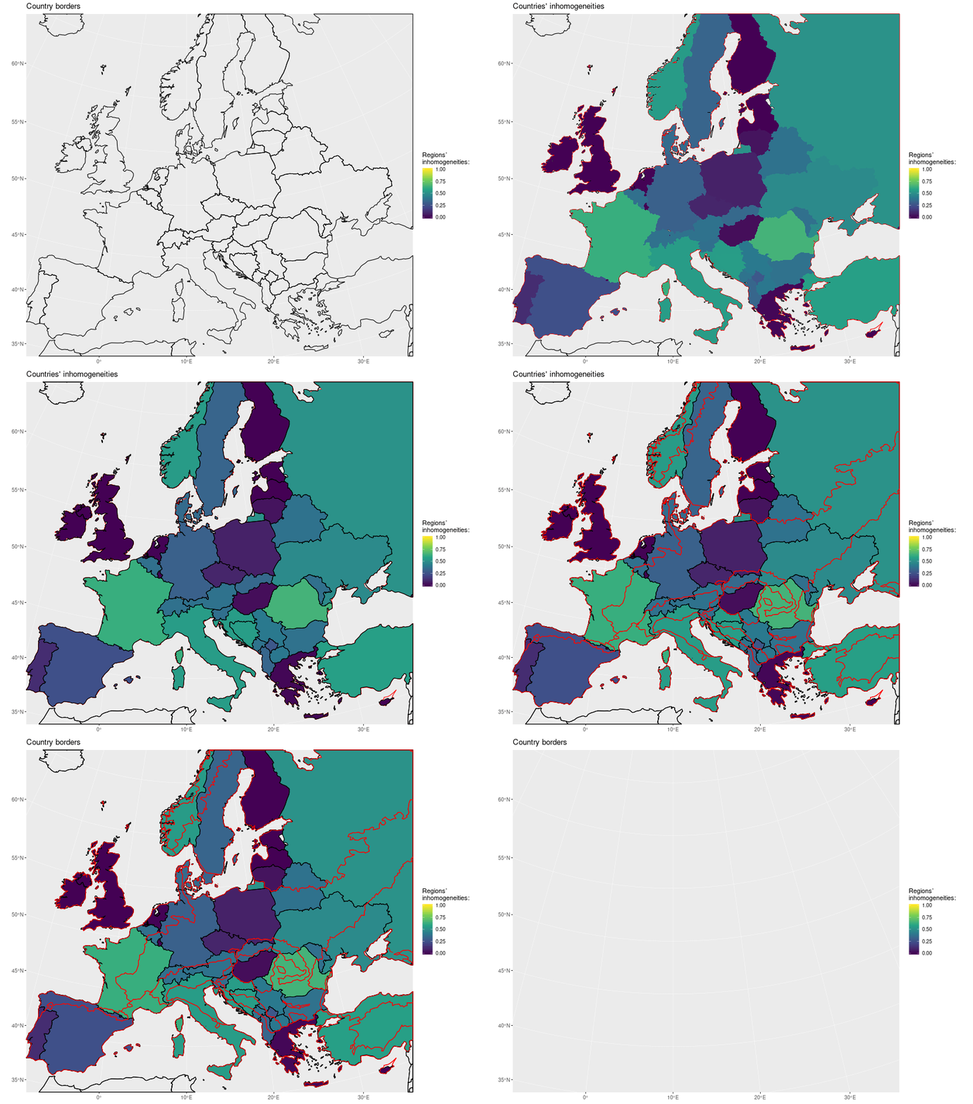
##  $map2 - the second map

V-measure, homogeneity, and completeness are global measures of association between the two regionalizations. Additional two maps indicate local associations by presenting regions’ inhomogeneities (rih). The first map shows how inhomogenous are countries with respect to biogeographical regions. For example, inhomogeneity of the Netherlands is zero as the country lies in only one biogeographical region and inhomogeneity of France is 0.63 as the country is divided by four different biogeographical regions. This measure also takes the area of biogeographical regions that cover each country into consideration. Both Poland and Belarus have two biogeographical regions, however in Poland, one region dominates the country area (rih = 0.08) and Belarus is almost equally divided by two regions (rih = 0.38).

A map of inhomogeneity of countries in terms of biogeographical regions

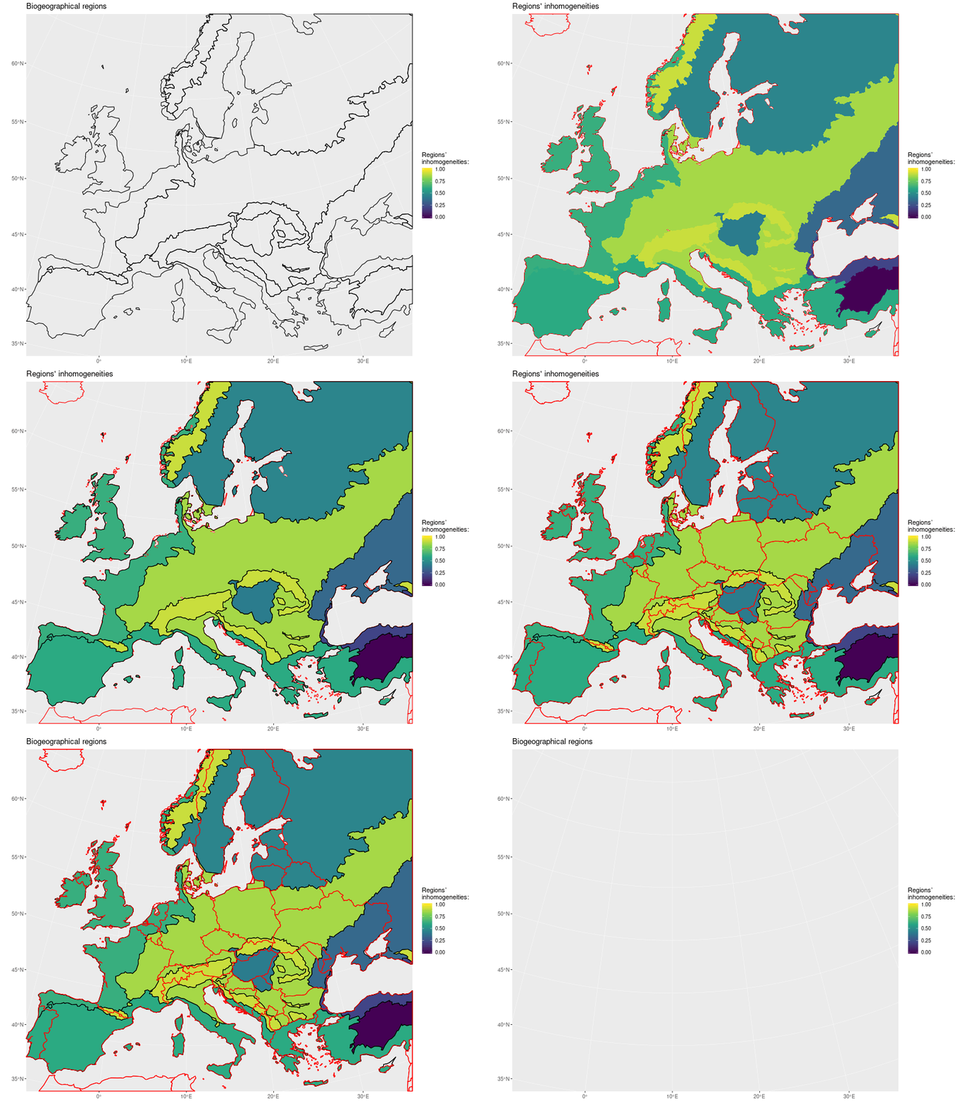
The second map represents how inhomogenous biogeographical regions are with respect to countries:

A map of inhomogeneity of biogeographical regions in terms of countries

Additional applications

This blog post focuses on providing the basic understanding of the spatial association between regionalizations. However, this method has a broader spectrum of possible applications, which we divide into three basic groups: comparative, associative, and derivative. In this blog post, we show an example of the comparative context. The associative context is used when you need to asses a degree of correspondence between a map of regions and maps of possible influencing factors. The role of derivative context is to help to select a number of spatial clusters. To learn more about all of these contexts take a look at our paper “Spatial association between regionalizations using the information-theoretical V-measure”. A freely available preprint is at https://eartharxiv.org/rcjh7/.

Quick summary

Spatial Association Between REegionalizations, sabre, is a spatial method adapted from computer science. It allows for three main types of analysis - comparative (comparison of regions), associative (relation between a regionalization and factor maps), and derivative (obtaining an optimal number of clusters). We implemented this method as an open-source software - an R package called sabre. This package allows for comparisons of maps in a form of vector objects. Let us know if you also want a support for raster map using the GitHub issue. To learn more you can visit the package website, read the original V-measure paper or our article “Spatial association between regionalizations using the information-theoretical V-measure”.