library(raceland)
library(raster)
library(sf)
library(tmap)
library(dplyr)The raceland package implements a computational framework for a pattern-based, zoneless analysis and visualization of (ethno)racial topography.
The main concept in this package is a racial landscape (RL). It consists of many large and small patches (racial enclaves) formed by adjacent raster grid cells having the same race categories. The distribution of racial enclaves creates a specific spatial pattern, which can be quantified by two metrics (entropy and mutual information) derived from the Information Theory concept (IT). Entropy is the measure of racial diversity and mutual information measures racial segregation.
Methods in the raceland package are based on the raster data, and unlike the previous methods, do not depend on the division for specific zones (census tract, census block, etc.). Calculation of racial diversity (entropy) and racial segregation (mutual information) can be performed for the whole area of interests (i.e., metropolitan area) or any portion of the whole area without introducing any arbitrary divisions.
To learn more about this topic, read our Applied Geography article or its preprint:
Dmowska, A., Stepinski T., Nowosad J. Racial landscapes – a pattern-based, zoneless method for analysis and visualization of racial topography. Applied Geography. 122:1-9, DOI:10.1016/j.apgeog.2020.102239
Example calculations
To reproduce the results on your own computer, install and attach the following packages:
You also need to download and extract the data.zip file containing the example data.
temp_data_file = tempfile(fileext = ".zip")
download.file("https://github.com/Nowosad/raceland-bp1/raw/master/data.zip",
              destfile = temp_data_file,
              mode = "wb")
unzip(temp_data_file)
Input data
The presented approach requires a set of rasters, where each raster represents one of five race-groups: Asians, Blacks, Hispanic, others, and Whites. In this example, we use data limited to the city of Cincinnati, Ohio.
list_raster = dir("data", pattern = ".tif$", full.names = TRUE)
race_raster = stack(list_raster)
We also use vector data containing the city borders to ease the understanding of the results.
cincinnati = read_sf("data/cincinnati.gpkg")We can visualize the data using the tmap package:
tm_race = tm_shape(race_raster) +
    tm_raster(style = "fisher",
              n = 10,
              palette = "viridis",
              title = "Number of people") +
    tm_facets(nrow = 3) +
    tm_shape(cincinnati) +
    tm_borders(lwd = 3, col = "black")
tm_race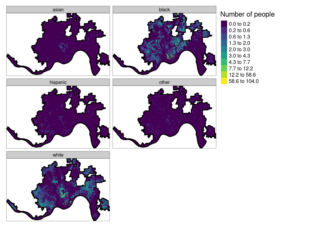
The above maps show the distribution of people from different race-groups in Cincinnati. Each, 30 by 30 meters, cell represents a number of people living in this area. Data was obtained from https://www.socscape.edu.pl/ and preprocessed using the instructions at https://cran.r-project.org/web/packages/raceland/vignettes/raceland-intro3.html.
Basic example
Our goal is to measure racial diversity and racial segregation for different places in the city. We can use the quantify_raceland() function for this purpose.
results_metrics = quantify_raceland(race_raster,
                                    n = 30,
                                    window_size = 10,
                                    fun = "mean",
                                    size = 20,
                                    threshold = 0.75)
head(results_metrics)
Simple feature collection with 6 features and 4 fields
Geometry type: POLYGON
Dimension: XY
Bounding box: xmin: 978285 ymin: 1858035 xmax: 984885 ymax: 1859235
CRS: PROJCRS["unknown",
BASEGEOGCRS["unknown",
DATUM["Unknown_based_on_GRS80_ellipsoid",
ELLIPSOID["GRS 1980",6378137,298.257222101004,
LENGTHUNIT["metre",1],
ID["EPSG",7019]]],
PRIMEM["Greenwich",0,
ANGLEUNIT["degree",0.0174532925199433,
ID["EPSG",9122]]]],
CONVERSION["Albers Equal Area",
METHOD["Albers Equal Area",
ID["EPSG",9822]],
PARAMETER["Latitude of false origin",23,
ANGLEUNIT["degree",0.0174532925199433],
ID["EPSG",8821]],
PARAMETER["Longitude of false origin",-96,
ANGLEUNIT["degree",0.0174532925199433],
ID["EPSG",8822]],
PARAMETER["Latitude of 1st standard parallel",29.5,
ANGLEUNIT["degree",0.0174532925199433],
ID["EPSG",8823]],
PARAMETER["Latitude of 2nd standard parallel",45.5,
ANGLEUNIT["degree",0.0174532925199433],
ID["EPSG",8824]],
PARAMETER["Easting at false origin",0,
LENGTHUNIT["metre",1],
ID["EPSG",8826]],
PARAMETER["Northing at false origin",0,
LENGTHUNIT["metre",1],
ID["EPSG",8827]]],
CS[Cartesian,2],
AXIS["easting",east,
ORDER[1],
LENGTHUNIT["metre",1,
ID["EPSG",9001]]],
AXIS["northing",north,
ORDER[2],
LENGTHUNIT["metre",1,
ID["EPSG",9001]]]]
row col ent mutinf geometry
30 1 30 1.0928666 0.01224849 POLYGON ((981885 1859235, 9...
31 1 31 1.2931567 0.03783377 POLYGON ((982485 1859235, 9...
33 1 33 1.1044932 0.01699973 POLYGON ((983685 1859235, 9...
34 1 34 1.6397933 0.05802896 POLYGON ((984285 1859235, 9...
74 2 24 0.9367936 0.01367241 POLYGON ((978285 1858635, 9...
80 2 30 1.4189221 0.04388582 POLYGON ((981885 1858635, 9...It requires several arguments:
x- RasterStack with race-specific population densities assign to each celln- a number of realizationswindow_size- expressed in the numbers of cells, is a length of the side of a square-shaped block of cells for which local densities will be calculatedfun- function to calculate values from adjacent cells to contribute to exposure matrix,"mean"- calculate average values of local population densities from adjacent cells,"geometric_mean"- calculate geometric mean values of local population densities from adjacent cells, or"focal"assign value from the focal cellsize- expressed in the numbers of cells, is a length of the side of a square-shaped block of cells. It defines the extent of a local patternthreshold- the share of NA cells to allow metrics calculation
The result is a spatial vector object containing areas of the size of 20 by 20 cells from input data (600 by 600 meters in this example). Its attribute table has five columns - row and col allowing for identification of each square polygon, ent - entropy measuring racial diversity, mutinf - mutual information, which is associated with measuring racial segregation, and geometry containing spatial geometries.
diversity_map = tm_shape(results_metrics) +
    tm_polygons(col = "ent",
                title = "Diversity",
                style = "cont",
                palette = "magma") +
    tm_shape(cincinnati) +
    tm_borders(lwd = 1, col = "black")
segregation_map = tm_shape(results_metrics) +
    tm_polygons(col = "mutinf",
                title = "Segregation",
                style = "cont",
                palette = "cividis") +
    tm_shape(cincinnati) +
    tm_borders(lwd = 1, col = "black")
tmap_arrange(diversity_map, segregation_map)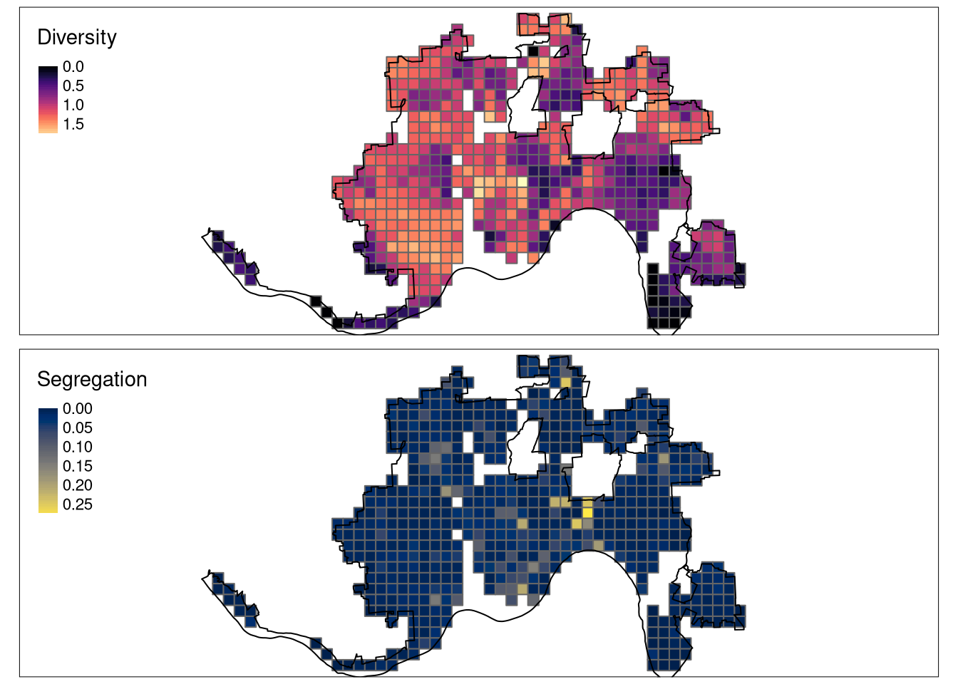
The above result present areas with different levels of racial diversity and segregation. Interestingly, there is a low correlation between these two properties. Some areas inside of the city do not have any value attached - this indicates either they are covered with missing values in more than 75% of their areas or nobody lives there.
Extended example
The quantify_raceland() function is a wrapper around several steps implemented in raceland, namely create_realizations(), create_densities(), calculate_metrics(), and create_grid(). All of them can be used sequentially, as you can see below.

Additionally, the raceland package has zones_to_raster() function that prepares input data based on spatial vector data with race counts.
Constructing racial landscapes
The racial landscape is a high-resolution grid in which each cell contains only inhabitants of a single race. It is constructed using the create_realizations() function, which expects a stack of race-specific rasters. Racial composition at each cell is translated into probabilities of drawing a person of a specific race from a cell. For example, if a cell has 100 people, where 90 are classified as Black (90% chance) and 10 as White (10% chance), then we can assign a specific race randomly based on these probabilities.
This approach generates a specified number (n = 30, in this case) of realization with slightly different patterns.
realizations_raster = create_realizations(race_raster, n = 30)The output of this function is a RasterStack, where each raster contains values from 1 to k, where k is a number of provided race-specific grids. In this case, we provided five race-specific grids (Asians, Blacks, Hispanic, others, and Whites), therefore the value of 1 in the output object represents Asians, number 2 Blacks, etc.
my_pal = c("#F16667", "#6EBE44", "#7E69AF", "#C77213", "#F8DF1D")
tm_realizations = tm_shape(realizations_raster[[1:4]]) +
    tm_raster(style = "cat",
              palette = my_pal,
              labels = c("Asians", "Blacks", "Hispanic", "others", "Whites"),
              title = "") +
    tm_facets(ncol = 2) +
    tm_shape(cincinnati) +
    tm_borders(lwd = 3, col = "black") +
    tm_layout(panel.labels = paste("Realization", 1:30))
tm_realizations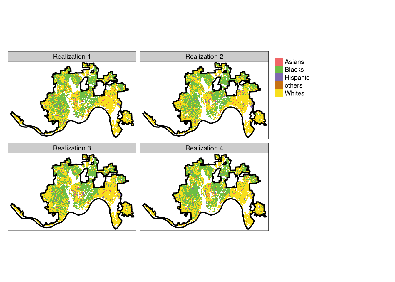
The above plot shows four of 30 created realizations and makes it clear that all of them are fairly similar.
Local densities
Now, for each of the created realization, we can calculate local densities of subpopulations (race-specific local densities) using the create_densities() function.
dens_raster = create_densities(realizations_raster,
                               race_raster,
                               window_size = 10)
The output is a RasterStack with local densities calculated separately for each realization.
tm_density = tm_shape(dens_raster[[1:4]]) +
    tm_raster(style = "fisher",
              n = 10,
              palette = "viridis",
              title = "Number of people") +
    tm_facets(ncol = 2) +
    tm_shape(cincinnati) +
    tm_borders(lwd = 3, col = "black") +
    tm_layout(panel.labels = paste("Realization", 1:30))
tm_density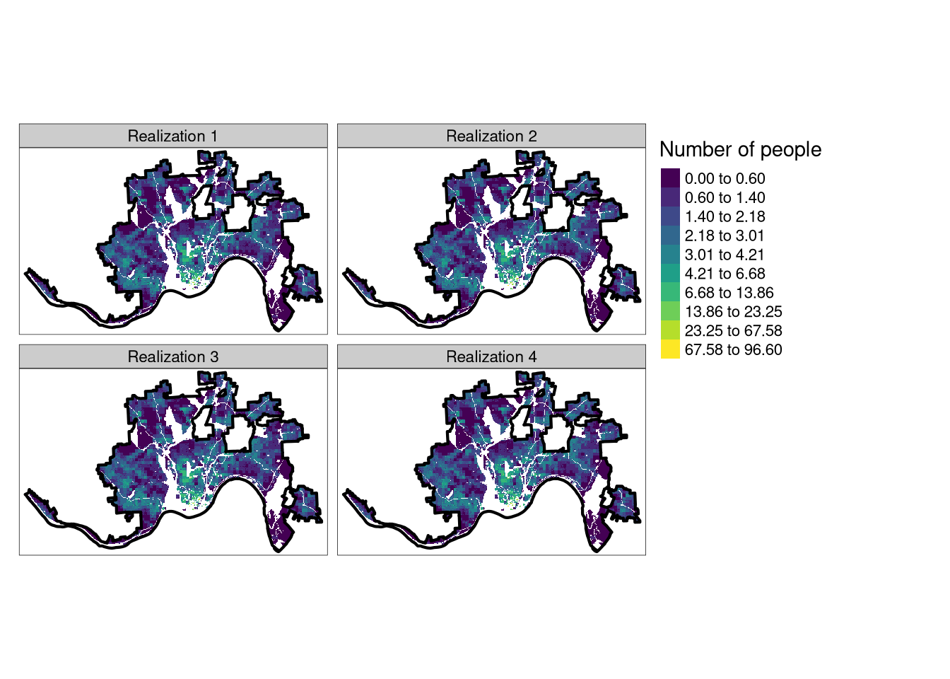
Total diversity and segregation
We can use both, realizations and density rasters, to calculate racial diversity and segregation using calculate_metrics() function. It calculates four information theory-derived metrics: entropy (ent), joint entropy (joinent), conditional entropy (condent), and mutual information (mutinf). As we mentioned before, ent is measuring racial diversity, while mutinf is associated with racial segregation. These metrics can be calculated for a given spatial scale. For example, setting size to NULL, as in the example below, calculates the metrics for the whole area of each realization.
metr_df = calculate_metrics(x = realizations_raster,
                            w = dens_raster,
                            fun = "mean",
                            size = NULL,
                            threshold = 1)
head(metr_df)
realization row col ent joinent condent mutinf
1 1 1 1 1.394937 2.617351 1.222414 0.1725237
2 2 1 1 1.395346 2.618786 1.223440 0.1719062
3 3 1 1 1.397898 2.621963 1.224065 0.1738325
4 4 1 1 1.397268 2.622896 1.225628 0.1716395
5 5 1 1 1.396112 2.617471 1.221359 0.1747527
6 6 1 1 1.398692 2.624289 1.225597 0.1730954Now, we can calculate average metrics across all realization, which should give more accurate results.
metr_df %>%
  summarise(
    mean_ent = mean(ent, na.rm = TRUE),
    mean_mutinf = mean(mutinf)
  )
mean_ent mean_mutinf
1 1.3984 0.1740535These values could be compared with values obtained by other US cities to evaluate, which cities have high average racial diversity (larger values of mean_ent) and which have high average racial segregation (larger values of mean_mutinf).
Local diversity and segregation
The information theory-derived metrics can be also calculated for smaller, local scales using the size argument. It describes the size of a local area for metrics calculations. For example, size = 20 indicates that each local area will consist of 20 by 20 cells of the original raster.
metr_df_20 = calculate_metrics(x = realizations_raster,
                               w = dens_raster,
                               fun = "mean",
                               size = 20,
                               threshold = 0.75)
Now, we can summarize the results for each local area independently (group_by(row, col)).
smr = metr_df_20 %>%
  group_by(row, col) %>%
  summarize(
    ent_mean = mean(ent, na.rm = TRUE),
    mutinf_mean = mean(mutinf, na.rm = TRUE),
  ) %>%
  na.omit()
head(smr)
# A tibble: 6 × 4
# Groups: row [2]
row col ent_mean mutinf_mean
<dbl> <dbl> <dbl> <dbl>
1 1 30 1.08 0.0154
2 1 31 1.31 0.0356
3 1 33 1.12 0.0166
4 1 34 1.62 0.0552
5 2 24 0.951 0.0163
6 2 30 1.44 0.0494Each row in the obtained results relates to some spatial locations. We can create an empty grid with appropriate dimensions using the create_grid() function. Its size argument expects the same value as used in the calculate_metrics() function.
grid_sf = create_grid(realizations_raster, size = 20)The result is a spatial vector object with three columns: row and col allowing for identification of each square polygon, and geometry containing spatial geometries.
tm_shape(grid_sf) +
    tm_polygons()
The first two columns,row and col, can be used to connect the grid with summary results.
grid_attr = dplyr::left_join(grid_sf, smr, by = c("row", "col"))
grid_attr = na.omit(grid_attr)
Finally, we are able to create two maps. The first one represents racial diversity (larger the value, larger the diversity; the ent_mean variable) and the second one shows racial segregation (larger the value, larger the segregation; the ent_mean variable).
diversity_map = tm_shape(grid_attr) +
    tm_polygons(col = "ent_mean",
                title = "Diversity",
                style = "cont",
                palette = "magma") +
    tm_shape(cincinnati) +
    tm_borders(lwd = 3, col = "black")
segregation_map = tm_shape(grid_attr) +
    tm_polygons(col = "mutinf_mean",
                title = "Segregation",
                style = "cont",
                palette = "cividis") +
    tm_shape(cincinnati) +
    tm_borders(lwd = 3, col = "black")
tmap_arrange(diversity_map, segregation_map)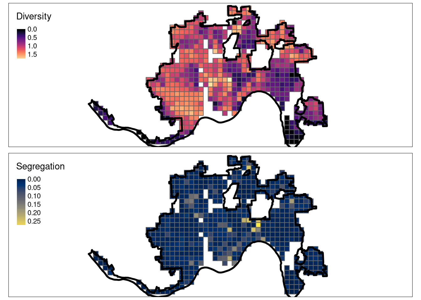
Bonus: visualizing racial landscapes
While the realizations created few steps before represents race spatial distribution fairly well, they do not take the spatial variability of the population densities into consideration. Additional function plot_realization() displays a selected realization taking into account not only race spatial distribution, but also the population density.
plot_realization(x = realizations_raster[[2]],
                 y = race_raster,
                 hex = my_pal)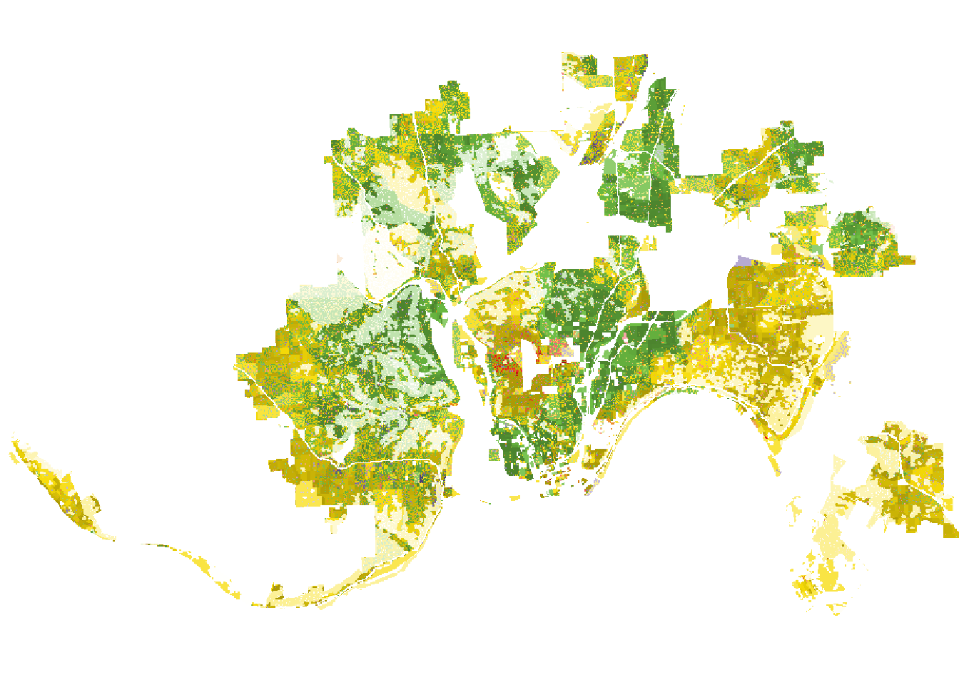
In its result, darker areas have larger populations, and brighter represent areas less-inhabited areas.
Summary
The raceland package implements a computational framework for a pattern-based, zoneless analysis and visualization of (ethno)racial topography. The most comprehensive description of the method can be found in the Racial landscapes – a pattern-based, zoneless method for analysis and visualization of racial topography article published in Applied Geography. Its preprint is available at https://osf.io/preprints/socarxiv/mejz5. Additionally, raceland has three extensive vignettes:
- raceland: R package for a pattern-based, zoneless method for analysis and visualization of racial topography - introducing the package and its functions
- raceland: Describing local racial patterns of racial landscapes at different spatial scales - showing how the calculations can be performed at different spatial scales
- raceland: Describing local pattern of the racial landscape using SocScape grids - presenting how to use the raceland methods with SocScape race-specific grids to perform analysis for different spatial scales, using the Cook county as an example.
This approach is based on the concept of ‘landscape’ used in the domain of landscape ecology. To learn more about information theory metrics used in this approach you can read the Information theory as a consistent framework for quantification and classification of landscape patterns article published in Landscape Ecology.
The raceland package requires race-specific grids. They can be obtained in two main ways. The first one is to download prepared grids from the SocScape project. It provides high-resolution raster grids for 1990, 2000, 2010 years for 365 metropolitan areas and each county in the conterminous US. The second way is to rasterize a spatial vector file (e.g., an ESRI Shapefile) with an attribute table containing race counts for some areas using the zones_to_raster() function.
Finally, while the presented methods have been applied to race-specific raster grids, they can be also used for many other problems where it is important to determine spatial diversity and segregation.
Reuse
Citation
@online{nowosad2020,
  author = {Nowosad, Jakub},
  title = {How to Measure Spatial Diversity and Segregation?},
  date = {2020-08-03},
  url = {https://jakubnowosad.com/posts/2020-08-03-raceland-bp1/},
  langid = {en}
}
