
![]()
TLTR:
Finding similar spatial patterns requires data for a query region and a search space. Spatial signatures are derived for the query region and many sub-areas of the search space, and distances between them are calculated. Sub-areas with the smallest distances from the query region are the most similar to it.
To reproduce the calculations in the following post, you need to download all of relevant datasets using the code below:
library(osfr)
dir.create("data")
osf_retrieve_node("xykzv") %>%
        osf_ls_files(n_max = Inf) %>%
        osf_download(path = "data",
                     conflicts = "overwrite")
You should also attach the following packages:
library(sf)
library(stars)
library(tmap)
Suwalski Landscape Park
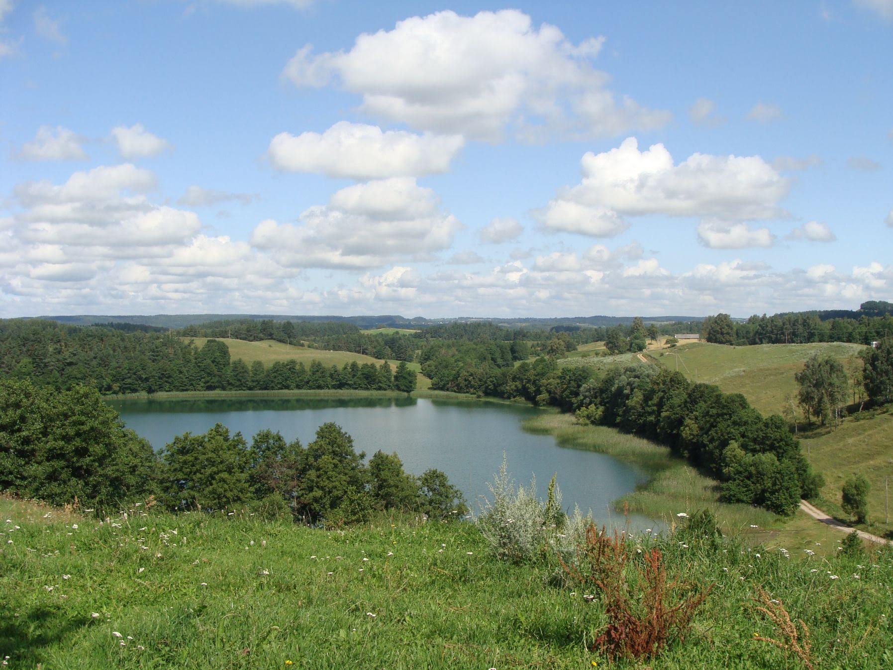
Spatial pattern search allows for quantifying similarity between the query region and the search space and finally finding regions that are the most similar to the query one. Here, we were interested in finding areas of similar topography to the area of Suwalski Landscape Park. Suwalski Landscape Park is a protected area in north-eastern Poland with a post-glacial landscape consisting of young morainic hills.
One possible approach to classify the topography of a given region is to use geomorphons. Geomorphons categorize cells in this area into one of ten forms: flat, summit, ridge, shoulder, spur, slope, hollow, footslope, valley, and depression 1.
The "data/geomorphons_pol.tif" file contains a raster with geomorphons calculated for Poland’s area, while "data/suw_lp.gpkg" is a vector polygon with the Suwalski Landscape Park borders. Let’s start by reading these two files into R.
gm = read_stars("data/geomorphons_pol.tif")
suw_lp = read_sf("data/suw_lp.gpkg")
Now, we can visualize geomorphons and the location of Suwalski Landscape Park with the tmap.
tm_gm = tm_shape(gm) +
        tm_raster(title = "Geomorphons:") +
        tm_shape(suw_lp) +
        tm_symbols(col = "black", shape = 6) +
        tm_layout(legend.outside = TRUE, frame = FALSE)
tm_gm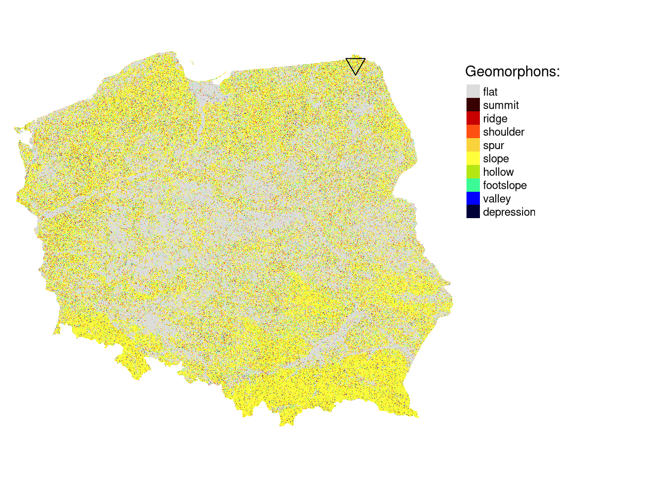
Search area
The geomorphon data for Poland is our search space. Now, we also need a second raster object with a query region. The query region is an area to which we want to find other similar areas.
There are two main ways to create a query region:
- By cropping spatial data of a large area to the extent or borders of a query region.
- By reading an external file. In the second case, the values in the external file should match the values in the search space.
Here, we are using the former approach by reading the Suwalski Landscape Park borders and then using it to crop the whole-country raster.
suw_lp = read_sf("data/suw_lp.gpkg")
gm_suw = st_crop(gm, suw_lp)
The query area has irregular spatial patterns represented by slopes and a limited number of flat areas.
tm_gm_suw = tm_shape(gm_suw) +
        tm_raster() +
        tm_shape(suw_lp) +
        tm_borders(col = "black") +
        tm_layout(legend.show = FALSE, frame = FALSE)
tm_gm_suw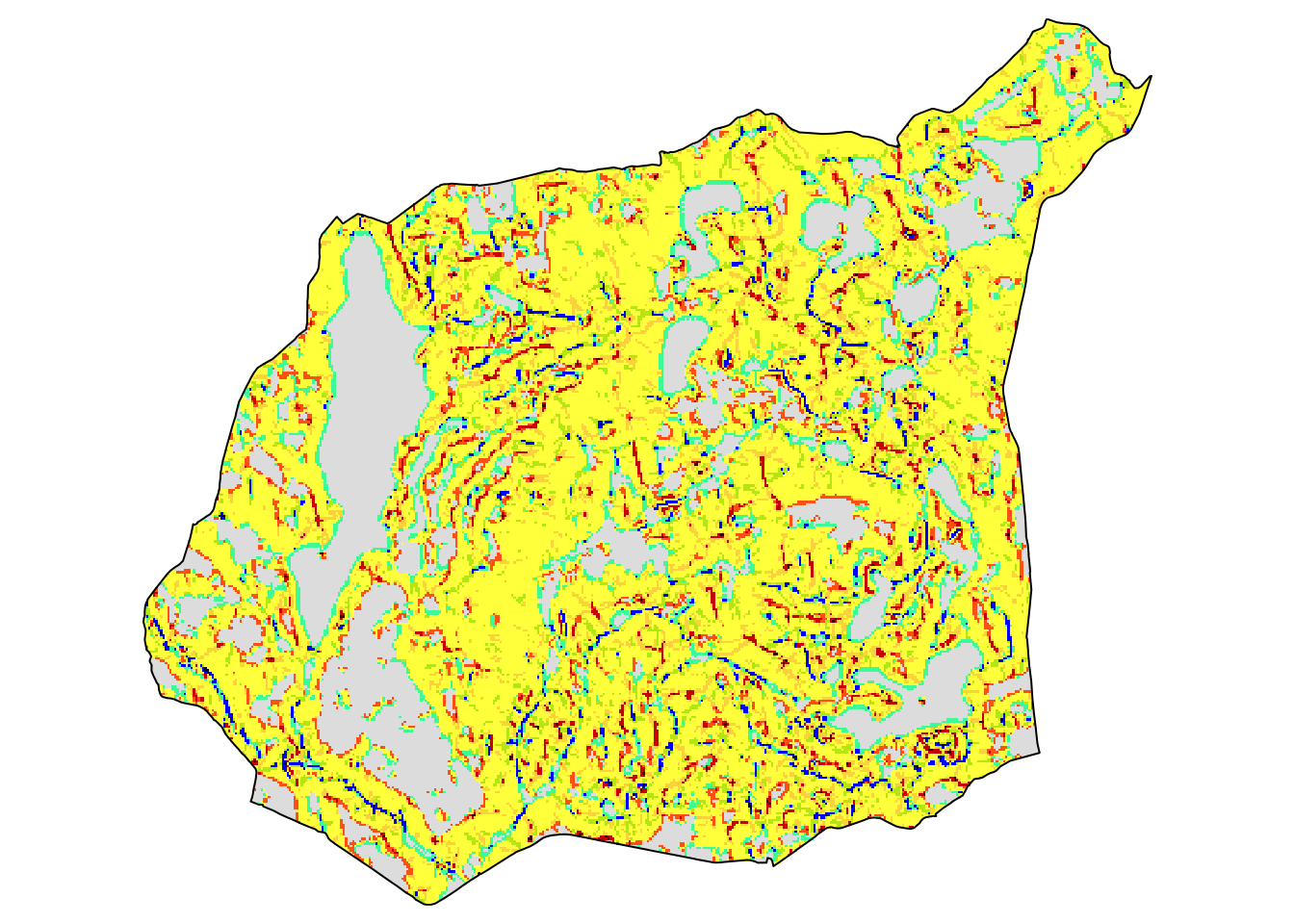
Search process
The searching process consists of:
- Selecting a query region and a search space. In our case, the query region is
gm_sum, while the search space is thegmobject. - Dividing the search space using regular (non-overlapping) squares or using polygons.
- Creating numerical representation (called a signature) for the query region and the search space.
- Comparing the signature of the query region with signatures for each part of the search space using a distance measure.
Search scale
The first important consideration is the search scale - what is the size of areas we want to find? This is not an easy question and largely depends on the research problem. The current version of motif accepts either regular (non-overlapping) squares or polygons.
Search signature
The second consideration is the search signature. We are able to describe the above area in words, however, how to translate the spatial pattern properties to a computer and, at the same time, made them more objective? Again, it is a complex question, and largely depends on the type of input data.
In our case, we have a single categorical raster, and for this type of data, we found out that the cove signature works well. Cove stands for co-occurrence vector - it is a 1D vector where each value represents what is the share of one category is adjacent to some other cells2. More information about cove can be found in the previous blog post.
We can calculate cove for our query region using lsp_signature() with the type argument set to "cove".
library(motif)
gm_sum_sig = lsp_signature(gm_suw, type = "cove")
gm_sum_sig
# A tibble: 1 × 3
id na_prop signature
* <int> <dbl> <list>
1 1 0.381 <dbl [1 × 100]>The output object contains a signature column, which stores the cove signature for our region. We can see this signature with gm_sum_sig$signature[[1]].
Search distance
The third consideration is a distance measure. Many distance measures have been developed for different types of data, and each of them has different properties. The motif package allows using any distance measure implemented in the philentropy package, which includes more than 40 different measures3.
Searching
The lsp_search() function performs spatial pattern-based search. It expects two stars objects: a query region (gm_suw) and a search space (gm). Next, we need to specify the search scale (window), signature (type), and distance method (dist_fun).
In this example, we use a window of 100 cells by 100 cells (window = 100). This means that our search scale will be 2500 meters (100 cells x data resolution) - resulting in dividing the search space into about 70,000 regular rectangles of 2500 by 2500 meters. We also use the "cove" signature and the "jensen-shannon" distance here.
gm_search = lsp_search(gm_suw, gm,
                       window = 100,
                       type = "cove",
                       dist_fun = "jensen-shannon")
The above calculation could take several minutes on a modern computer.
Search results
By default, the output of the search is a stars object with three attributes:
id- an id of each window,na_prop- share between 0 and 1 of NA cells for each window in the search space,dist- derived distance between the query region and each window in the search space.
gm_searchstars object with 2 dimensions and 3 attributes
attribute(s):
Min. 1st Qu. Median Mean 3rd Qu.
id 1.000000000 1.764075e+04 3.528050e+04 3.528050e+04 5.292025e+04
na_prop 0.000000000 0.000000e+00 0.000000e+00 3.111193e-03 0.000000e+00
dist 0.001737701 4.483980e-02 1.051218e-01 1.461936e-01 2.080158e-01
Max. NA's
id 7.056000e+04 0
na_prop 4.997000e-01 20485
dist 6.451746e-01 20485
dimension(s):
from to offset delta refsys point values x/y
x 1 288 4595300 2500 +proj=laea +lat_0=52 +lon... NA NULL [x]
y 1 245 3556600 -2500 +proj=laea +lat_0=52 +lon... NA NULL [y]We can visualize the result in the same fashion as a regular stars object (see the final map at the end of the post):
tm_search2 = tm_shape(gm_search) +
          tm_raster("dist",
                  style = "log10",
                  palette = "BrBG",
                  title = "Distance (JSD):",
                  legend.is.portrait = FALSE)
A search result can also be easily converted into an sf object with st_as_sf(). This allows for straightforward analysis and subsetting of the search results.
gm_search_sf = st_as_sf(gm_search)The most similar areas
Spatial pattern-based search is similar to a search using internet search engines - we do not care about the most dissimilar areas. We just want to locate the ones most similar to the query region. Therefore, we should select only areas with the smallest distance values - this means that they are the most similar to the query region.
We can achieve it, for example, using the slide_min() function. The code below selects nine areas with the smallest distance from the query region.
library(dplyr)
gm_search_sel = slice_min(gm_search_sf, dist, n = 9)
If we want to look closer at the result, then we can extract each of the above regions with the lsp_add_examples() function. It adds a region column with a stars object to each row.
gm_search_ex = lsp_add_examples(x = gm_search_sel, y = gm)It allows us to visualize any of the most similar areas.
tm_shape(gm_search_ex$region[[1]]) +
  tm_raster() +
  tm_layout(legend.show = FALSE)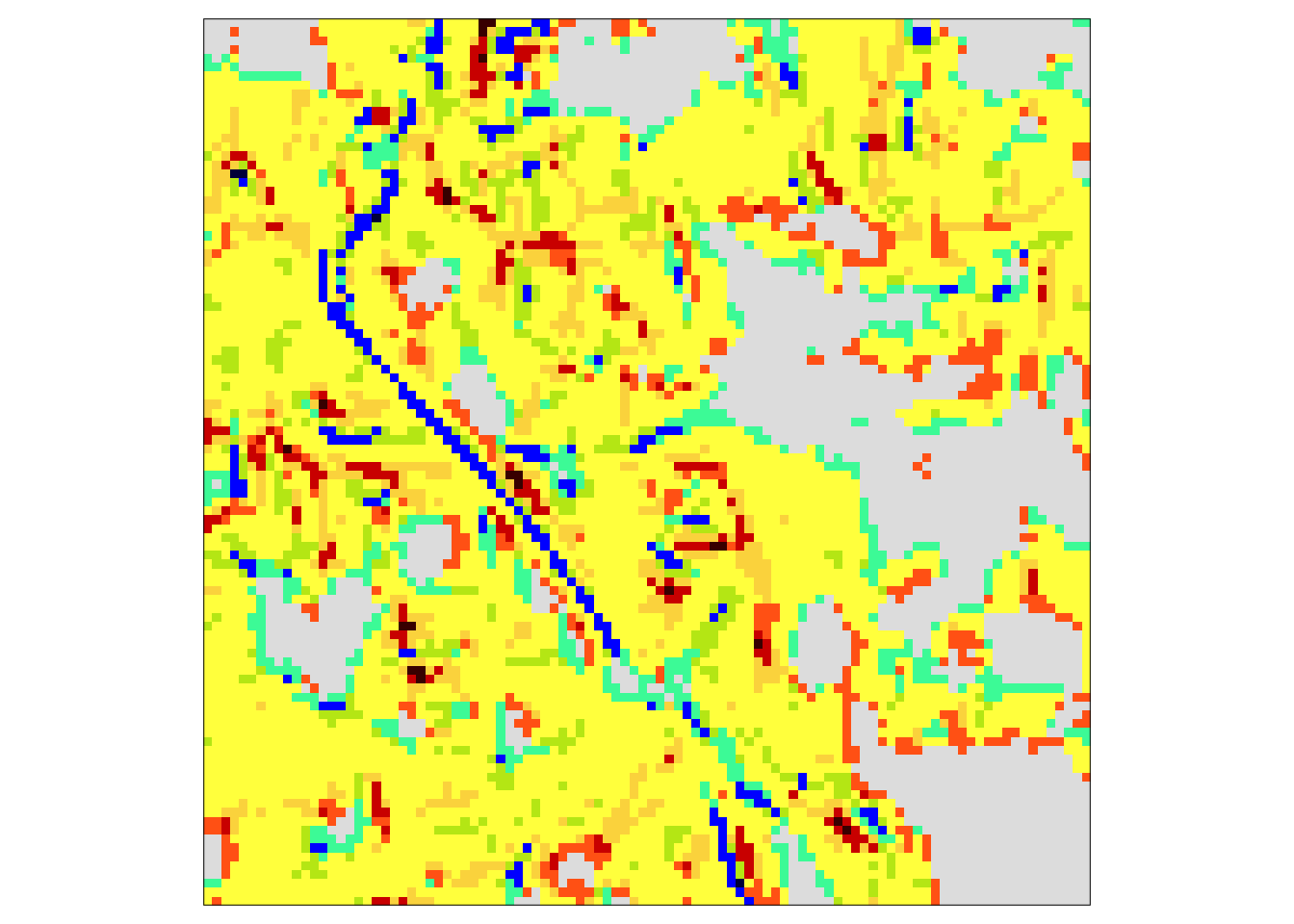
This approach can also be extended to plot all nine of the most similar areas. We just need to create a visualization function (create_map()) and use it iteratively on each region in gm_search_ex. The output of this process, map_list, is a list of tmaps that can be plotted with tmap_arrange():
library(purrr)
create_map = function(x, y){
  tm_shape(x) +
  tm_raster() +
  tm_layout(legend.show = FALSE,
            title = y)
}
map_list = map2(gm_search_ex$region, gm_search_ex$id, create_map)
tmap_arrange(map_list)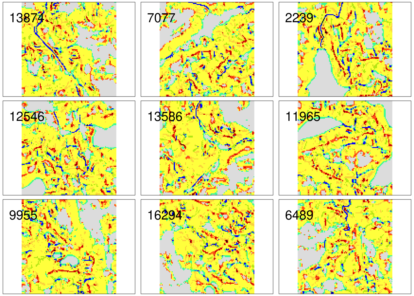
Nine examples of the areas with the most similar patterns of geomorphons comparing to the Suwalski Landscape Park are presented above. They are also similar to each other, suggesting a high-quality result.
The final map consists of two parts: (a) a distance raster and (b) symbols representing the nine most similar areas.
tm_search2 +
  tm_shape(gm_search_sel) +
  tm_symbols(shape = 2, col = "black") +
  tm_text("id", auto.placement = TRUE)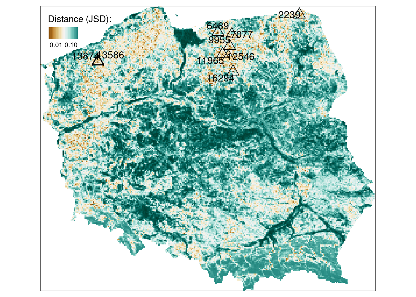
The brown color on the above map represents areas with the most similar patterns of geomorphons to the Suwalski Landscape Park. The majority of similar areas are located in northern Poland and forms a belt with homogeneous topography.
Summary
The pattern-based search allows for finding areas with similar spatial patterns. The above example shows the search based on a single variable raster data (geomorphons), but by using a different spatial signature, it can be performed on rasters with two or more variables. Additionally, search space can be not only divided into regular areas, but also in irregular ones - see an example. R code for the pattern-based search can be found here.
Footnotes
Learn more about geomorphons by reading the dedicated paper or its preprint. You can also calculate geomorphons for your own data using a GRASS GIS module r.geomorphon.↩︎
In other words, it is a vector containing a normalized form of the co-occurrence matrix.↩︎
You can check all of them using
philentropy::getDistMethods().↩︎
Reuse
Citation
BibTeX citation:
@online{nowosad2021,
  author = {Nowosad, Jakub},
  title = {Finding Similar Spatial Patterns},
  date = {2021-02-17},
  url = {https://jakubnowosad.com/posts/2021-02-17-motif-bp3/},
  langid = {en}
}
For attribution, please cite this work as:
Nowosad, Jakub. 2021. “Finding Similar Spatial Patterns.”
February 17. https://jakubnowosad.com/posts/2021-02-17-motif-bp3/.