Quantifying changes of spatial patterns

TLTR:

Quantifying changes of spatial patterns requires two datasets for the same variable in the same area. Both datasets are divided into many sub-areas, and spatial signatures are derived for each sub-area for each dataset. Next, distances for each pair of areas are calculated. Sub-areas with the largest distances represent the largest change.

To reproduce the calculations in the following post, you need to download all of relevant datasets using the code below:

library(osfr)
dir.create("data")
osf_retrieve_node("xykzv") %>%
        osf_ls_files(n_max = Inf) %>%
        osf_download(path = "data",
                     conflicts = "overwrite")

You should also attach the following packages:

library(stars)
library(motif)
library(tmap)
library(readr)

Spatial patterns changes

A standard approach for detecting changes between two rasters is to calculate a change for each cell independently. This allows quantifying how cells changed their values for A to B, and how many from B to A. However, this approach does not tell us if the spatial pattern actually had changed or stayed the same. For example, consider a regular checkerboard and a checkerboard with all colors reversed. While every cell changed its value, we still have the classes, and their spatial arrangement is the same.

Here, we are interested in changes of spatial patterns, therefore, instead of looking at pixel-by-pixel change, we focus on pattern-by-pattern change ¹.

Land cover in the Amazon

The data/lc_am_1992.tif contains land cover data for the year 1992 and data/lc_am_2018.tif for the year 2018. Both are single categorical rasters of the same extent, the Amazon, and the same resolution - 300 meters that can be read into R using the read_stars() function.

lc92 = read_stars("data/lc_am_1992.tif")
lc18 = read_stars("data/lc_am_2018.tif")

Additionally, the data/lc_palette.csv file contains information about the colors and labels of each land cover category.

lc_palette_df = read_csv("data/lc_palette.csv")
names(lc_palette_df$color) = lc_palette_df$value

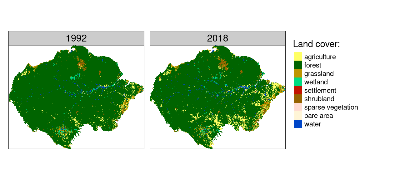
Both land cover dataset can be visualized with tmap. The lc_palette_df is used to set a color palette and legend’s labels.

tm_compare1 = tm_shape(c(lc92, lc18)) +
        tm_raster(style = "cat",
                  palette = lc_palette_df$color,
                  labels = lc_palette_df$label,
                  title = "Land cover:") +
        tm_layout(legend.outside = TRUE,
                  panel.labels = c(1992, 2018))
tm_compare1

The above map clearly shows that there has been a large land cover change in many areas of Amazon between 1992 and 2018. The problem now is to find out what areas changed the most.

Comparing spatial patterns

This could be solved with lsp_compare(). The lsp_compare() function expects two stars objects with the same extent and resolution. We also need to specify the spatial scale of comparison (window), signature (type), and distance method (dist_fun)².

In this example, we use a window of 300 cells by 300 cells (window = 300). This means that our search scale will be 90 km (300 cells x data resolution) - resulting in dividing the whole area into about 1,500 regular rectangles of 90 by 90 kilometers. We also use the "cove" signature and the "jensen-shannon" distance here.

lc_am_compare = lsp_compare(lc92, lc18, 
                            window = 300, 
                            type = "cove",
                            dist_fun = "jensen-shannon")

Comparing results

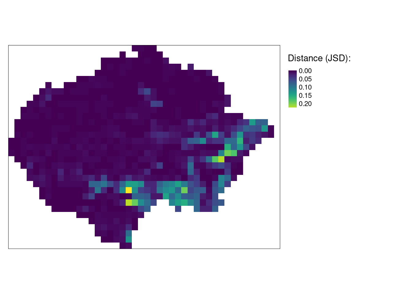
By default, the output is a stars object with four attributes: (1) id - an id of each window, (2) na_prop_x - share between 0 and 1 of NA cells for each window in the first stars object, (3) na_prop_y - share between 0 and 1 of NA cells for each window in the second stars object, (4) dist - derived distance between the pattern in the first object and the second object for each window.

lc_am_compare

stars object with 2 dimensions and 4 attributes
attribute(s):
           Min.      1st Qu.       Median         Mean      3rd Qu.
id            1 3.637500e+02 7.265000e+02 726.50000000 1.089250e+03
na_prop_x     0 0.000000e+00 0.000000e+00   0.02093060 0.000000e+00
na_prop_y     0 0.000000e+00 0.000000e+00   0.02112938 0.000000e+00
dist          0 1.504208e-03 3.550033e-03   0.01713996 1.100637e-02
                   Max. NA's
id         1452.0000000    0
na_prop_x     0.4933778  620
na_prop_y     0.4933778  620
dist          0.2469178  620
dimension(s):
  from to   offset  delta                       refsys point values x/y
x    1 44 -8834600  90000 Interrupted_Goode_Homolosine    NA   NULL [x]
y    1 33   964250 -90000 Interrupted_Goode_Homolosine    NA   NULL [y]

We can visualize the result the same as a regular stars object, for example using the tmap package:

tm_compare2 = tm_shape(lc_am_compare) +
        tm_raster("dist", 
                  palette = "viridis", 
                  style = "cont",
                  title = "Distance (JSD):") +
        tm_layout(legend.outside = TRUE)
tm_compare2

The yellow color represents areas of the largest change. They are mostly located in the south and south-east part of the Amazon.

A comparison result can also be easily converted into an sf object with st_as_sf() for subsetting and analyzing the outcomes.

lc_am_compare_sf = st_as_sf(lc_am_compare)

Areas of the largest change in the pattern

In the previous blog post, we were interested in finding the most similar areas to the query region - smallest distance. Here, we are looking for the areas with the largest change, which is expressed by the largest dist values.

We can use slice_max() to subset the obtained result to a selected number of areas with the largest change between 1992 and 2018. The code below selects nine areas with the largest distance between the spatial pattern in 1992 and 2018.

library(dplyr)
lc_am_compare_sel = slice_max(lc_am_compare_sf, dist, n = 9)

If we want to look closer at the result, then we can extract each of the above regions with the lsp_add_examples() function. It adds a region column with a stars object to each row.

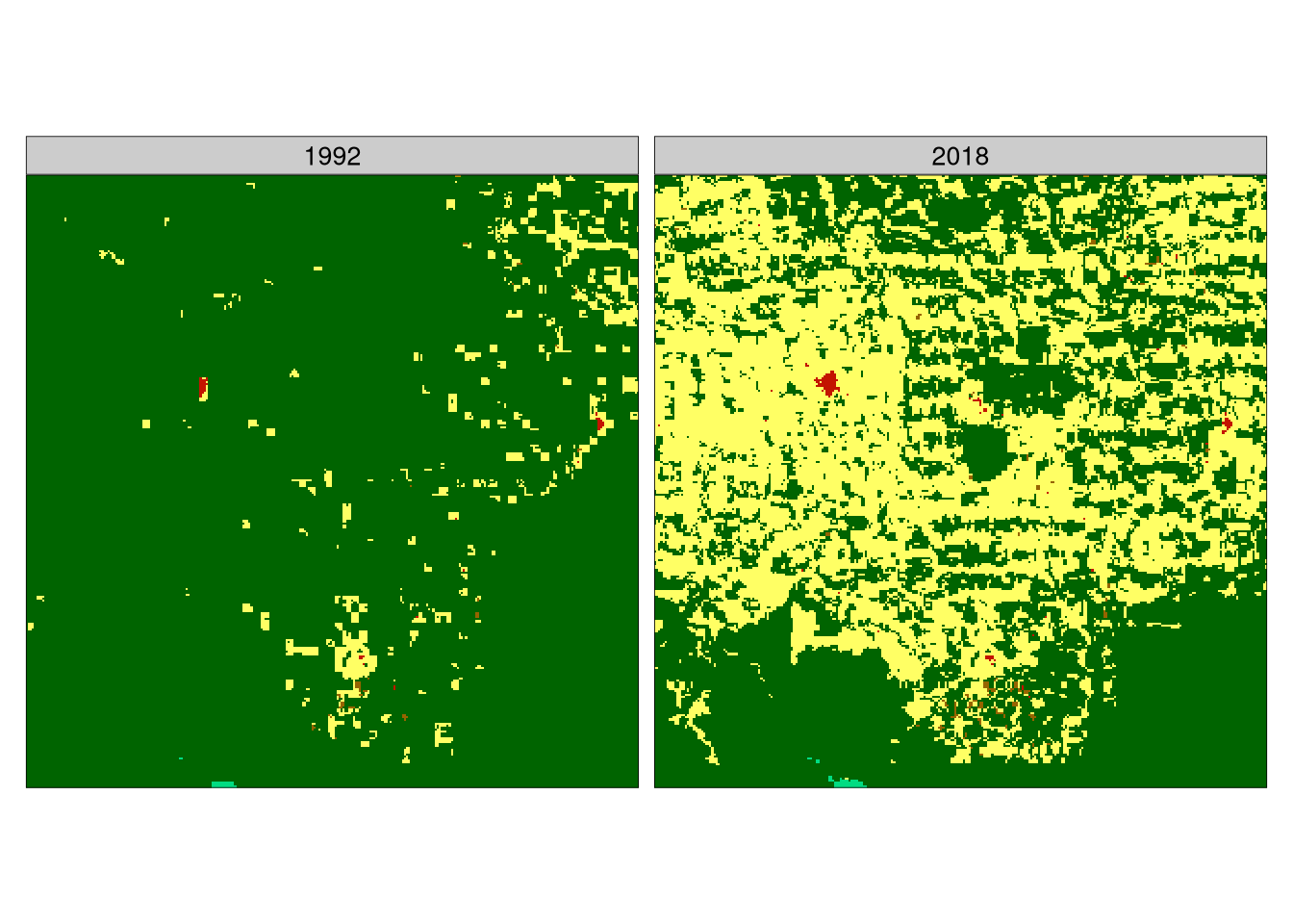
lc_am_compare_ex = lsp_add_examples(x = lc_am_compare_sel, y = c(lc92, lc18))

It allows us to visualize area with the largest change:

tm_shape(lc_am_compare_ex$region[[1]]) + 
  tm_raster(style = "cat",
                          palette = lc_palette_df$color,
                          labels = lc_palette_df$label,
                          title = "Land cover:") +
  tm_layout(legend.show = FALSE,
            panel.labels = c(1992, 2018))

Here, we can see an area mostly covered by forest in 1992, which large parts were transformed into agriculture before 2018.

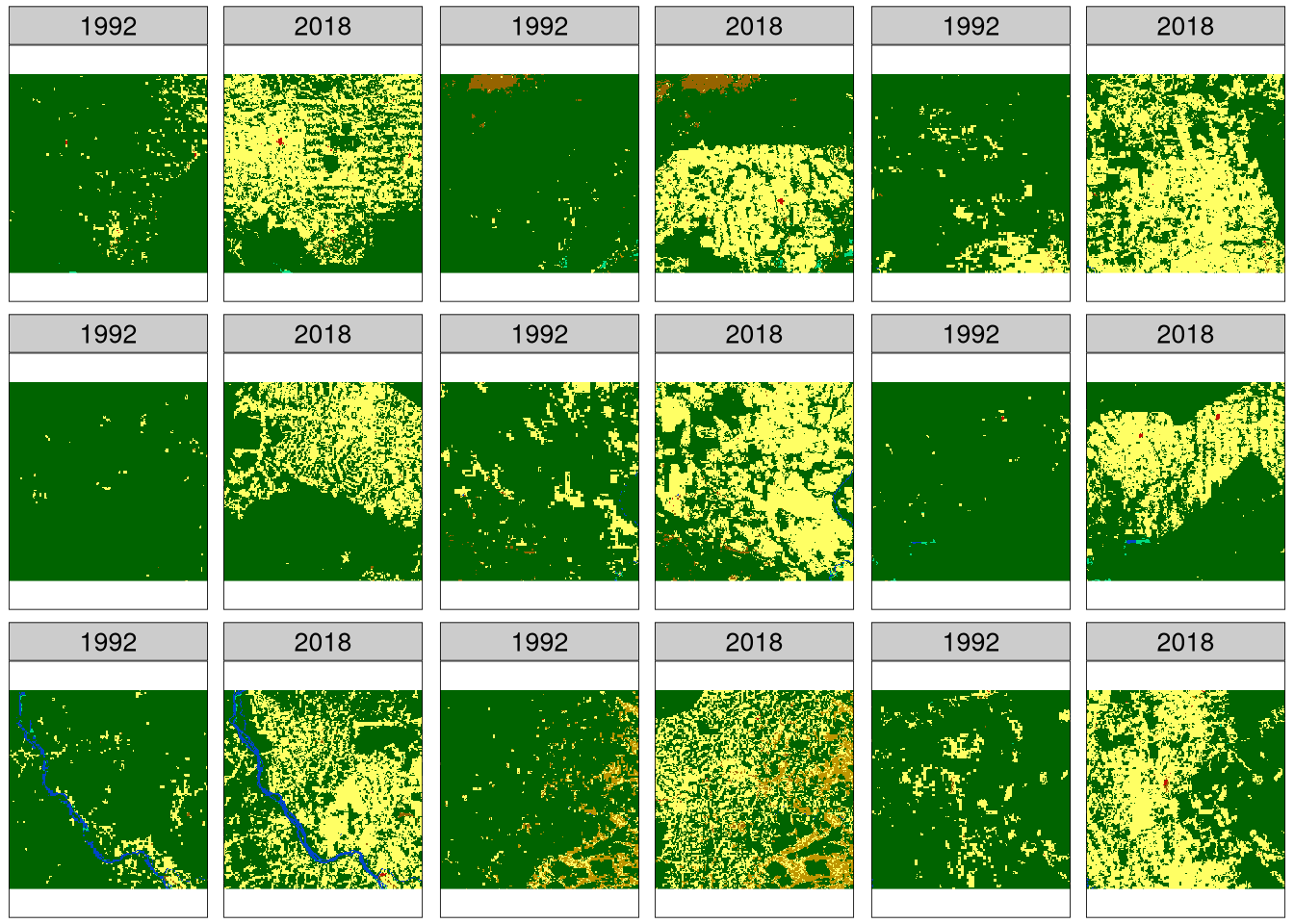
This approach can also be extended to plot all nine areas. We just need to create a visualization function (create_map2()) and use it iteratively on each region in lc_am_compare_ex. The output of this process, map_list, is a list of tmaps that can be plotted with tmap_arrange():

library(purrr)
create_map2 = function(x){
        tm_shape(x) +
                tm_raster(style = "cat",
                          palette = lc_palette_df$color,
                          labels = lc_palette_df$label,
                          title = "Land cover:") +
                tm_facets(ncol = 2) +
                tm_layout(legend.show = FALSE,
                          panel.labels = c(1992, 2018))
}
map_list = map(lc_am_compare_ex$region, create_map2)
tmap_arrange(map_list)

It shows that majority of changes in the Amazon are related to the forest being removed for agricultural purposes.

Summary

The pattern-based comparison allows for finding areas with the largest change in spatial patterns. The above example shows the search based on a single variable raster data (land cover), but by using a different spatial signature, it can be performed on rasters with two or more variables (think of multi-variable change). R code for the pattern-based comparison can be found here, with other examples described in the Spatial patterns’ comparision vignette.

Footnotes

1. For a more detailed explanation of spatial patterns’ changes, visit my older blog post.

2. If you want more explanation about these arguments, please read the previous posts in this series.