Considerations for the pattern-based spatial analysis

TLTR:

This is a last blog post in a series about motif - an R package aimed for pattern-based spatial analysis. It sums up previous posts, but also underlines potential considerations when working with spatial patterns. Finally, it lists underexplored topics and future ideas related to pattern-based spatial analysis.

Pattern-based spatial analysis

The first blog post in this series introduces a basic concept of categorical data spatial patterns, and why commonly used landscape metrics are not best suited for finding areas with similar spatial patterns. A better approach is to derive a spatial signature - a multi-number description that compactly stores information about the composition and configuration of a spatial pattern.

In the second blog post presents some basic spatial signatures, including coma (co-occurrence matrix) for single-variable categorical rasters, wecoma (weighted co-occurrence matrix) for single-variable categorical rasters that have another continuous raster representing the intensity of categories, and incoma (integrated co-occurrence matrix) for categorical rasters with two or more variables. All of the mentioned spatial signatures can be converted into a 1D vector - a probability function, and similarity between probability functions can be calculated using one of many distance measures (e.g., Jenson-Shannon distance). Now, having spatial signatures for two areas, we can find out how similar (or dissimilar) they are. This allows us to find the most similar rasters, describe changes between rasters, or group (cluster) rasters based on the spatial patterns.

The third blog post shows how we can search for areas with similar spatial patterns to a query region based on an example of finding areas of similar topography to the area of Suwalski Landscape Park. In the search process, spatial signatures are derived for the query region and many sub-areas of the search space, and distances between them are calculated. Next, sub-areas with the smallest distances from the query region are assumed to be the most similar to it.

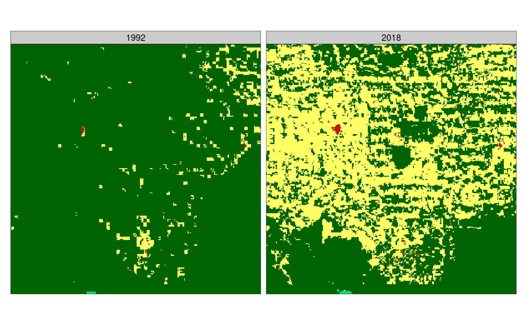
The fourth blog post focused on finding areas with the largest change of land cover patterns in the Amazon between 1992 and 2018. The land cover data from the Amazon in 1992 and 2018 were subdivided into areas of 90 by 90 kilometers, and a spatial signature was calculated for each subarea in each year. Then, a distance between spatial signatures for each subarea was derived, with large distance values indicating a large change of spatial patterns.

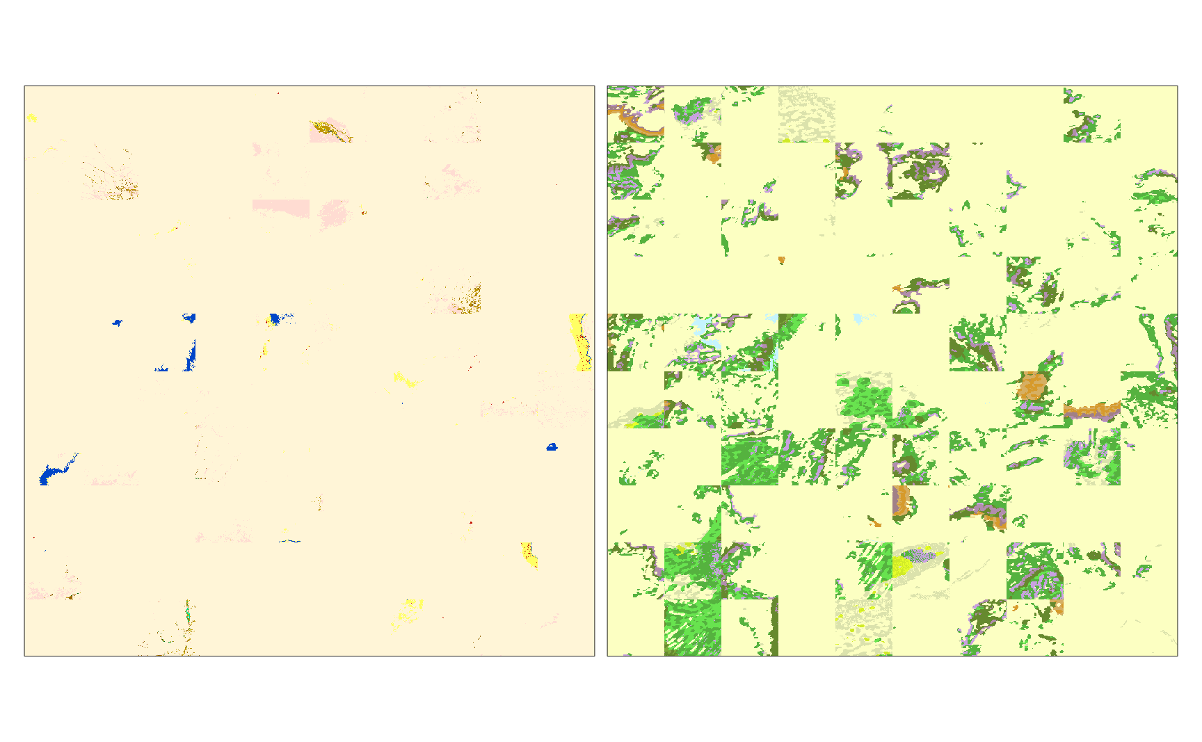
The fifth blog post showcases clustering of similar spatial patterns of joint spatial patterns of land cover and landforms in Africa. In this process, Africa was divided into many sub-areas and spatial signatures were derived for each sub-area. Distances between signatures for each sub-area were calculated and stored in a distance matrix, which was used as a basis for the creation of clusters of similar spatial patterns. The quality of clusters was assessed visually using a pattern mosaic and with dedicated quality metrics.

Potential applications

The role of the presented examples is to highlight the universality and extensibility of the pattern-based methods. They could be used in a wide range of local, regional, and global studies of global environmental changes, land management, sustainable development, environmental protection, forest cover change, urban growth monitoring, or agriculture expansion studies. Some example research ideas include:

• studying global environmental changes by analysis of changes in patterns of different environmental features, such as land cover,
• delineating of ecoregions - regionalization of land into homogeneous units of similar ecological and physiographic features (land cover, landform, soils, climate),
• clustering of forest patterns, which results could be used for conservation, planning, and management
• identifying spatial patterns of cropland usage
• inventorying of landscape patterns and analysis of landscape spatial configuration

Additionally, the pattern-based spatial analysis methods and tools could be useful in various other disciplines that use categorical images, for example, medical science, astronomy, or social studies.

Study considerations

However, no matter if we analyze patterns in an environmental raster, demographic map, or categorized microscope image, we need to consider several questions.

How should we preprocess the input data? For example, do we need all 18 categories in our data, or is it better to simplify the number of categories to improve analysis and streamline interpretation of the results? When we are interested in forest fragmentation, do we really need several other land cover classes, or can we merge them into one or two categories? Additionally, preprocessing can be applied to derive new categories from the data. An example of this was shown in the third blog post, where elevation data was first converted into geomorphons before applying any other steps. Reprojecting of the input data may also be important in some cases. In the pattern-based spatial analysis, each cell is treated equally, which means that we usually want to apply data in some equal-area projection.

What is the scale of the process we want to study? Are we interested in investigating patterns in 10 by 10 cell windows or maybe 100 by 100 cell windows? If we do not have any prior information or expectation about spatial scale, then there are two general approaches that could help. Firstly, we could apply the same analysis steps a few times using different sizes of a local window, and decide on a proper spatial scale afterward. Secondly, we could use the smallest meaningful windows we can think of¹, for example, 10 by 10 cells, and then apply the clustering process. After merging similar areas into larger regions, we can decide the spatial scale of homogeneous spatial patterns.

Which signature should we apply? The coma representation was developed for single-variable categorical rasters, wecoma for single-variable categorical rasters that have another continuous raster representing the intensity of categories, and incoma for categorical rasters with two or more variables. Which of the above representation suits your problem the best? Or maybe you need to create some new signature focused on the specifics of your case?

Which distance measure should we use? A few dozen of distance/dissimilarity measures exist². Our previous experiences showed that the Jensen-Shannon distance is suitable to describe relations between spatial patterns of land cover data. However, there is no free lunch in selecting a distance measure, and I would usually recommend trying out a few measures before deciding on one of them.

General considerations and future work

There are also general considerations that would gain from establishing a consistent methodology. For example, how to decide which scale is valid? What type of signatures are still missing and should be developed? How to integrate categorical and continuous spatial patterns in an analysis? What are the advantages and disadvantages of using different distance measures? What are the missing workflows that can be added to the pattern-based spatial analysis?

I encourage everyone to submit their issues or enhancement requests to the motif package, which will help me to prioritize my work. Furthermore, if you have any questions or ideas related to the pattern-based spatial analysis, please email me at nowosad.jakub@gmail.com.

Footnotes

1. This depends on the number of categories, their spatial arrangements, etc.

2. Read https://users.uom.gr/~kouiruki/sung.pdf for a comprehensive review of distance measures.