Spatial regionalization using universal superpixels algorithm

This is a second blog post in a series about the supercells package. You can read the first one at “supercells: universal superpixels algorithm for applications to geospatial data”.

The main idea of supercells is to create groupings of adjacent cells that share common characteristics. This process often results in an over-segmentation – a situation when supercells are internally homogeneous, but not very different from their neighbors. Thus, we need to find the best way to merge similar adjacent supercells into larger entities (regions). It can be done with various approaches, both supervised and unsupervised. Here, we will focus on two examples of unsupervised approaches. The first one, k-means, is a general clustering method, while the second one, SKATER, is a spatial clustering method. The main goals of this blog post are to show how the merging of supercells can be performed and how to evaluate the obtained results.

Example

Let’s start by attaching the packages and reading the input data. We will use the same packages as in the first blog post with one addition – dplyr.

library(supercells)
library(terra)
library(sf)
library(regional)
library(tmap)
library(dplyr)

Here, we will also use the same dataset cropped to an area of 50 by 100 cells.

flc = rast("/vsicurl/https://github.com/Nowosad/supercells-examples/blob/main/raw-data/all_ned.tif?raw=true")
flc1 = project(flc, "EPSG:3035", method = "near")
flc1 = flc[101:150, 1:100, drop = FALSE]

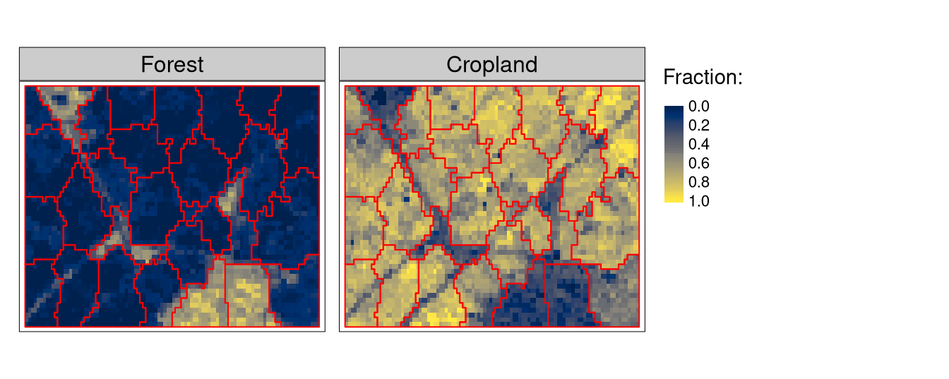
Our next preparation step will be to create a set of supercells representing areas with homogeneous arrangements of fractional land cover values (Figure 1).

flc_sc = supercells(x = flc1,
                    step = 12, compactness = 0.1,
                    dist_fun = "jensen-shannon")

tm_shape(flc1[[c(1, 5)]]) +
  tm_raster(style = "cont", palette = "cividis", title = "Fraction:") +
  tm_shape(flc_sc) +
  tm_borders(col = "red")

Figure 1: Supercells on the top of fractions of the forest and cropland classes

As a final preparation step, we will also calculate supercells areas and keep them in the area_km2 column.

flc_sc$area_km2 = as.numeric(st_area(flc_sc)) / 1000000

K-means

K-means clustering partitions observations into a selected number (k) of clusters. In our case, each observation is a supercell, and thus, each k-means cluster will represent a set of supercells. Notably, the k-means algorithm is unaware of spatial relationships in our data – it does not know that some supercells are adjacent to others. Therefore, clusters returned by the k-means algorithm may consist of many supercells located in different places in our area of interest.

To use the k-means algorithm, we need to extract only variables (columns) with fractional land cover values:

vars = c("Forest", "Shrubland", "Grassland", "Bare.Sparse.vegatation", 
         "Cropland", "Built.up", "Seasonal.inland.water",
         "Permanent.inland.water")
flc_sc_df = st_drop_geometry(flc_sc)[vars]

Then, we can apply the clustering by making one major decision – what is the expected number of clusters (k/the centers argument). For this example, I created four clusters:¹

set.seed(2022-11-10)
km_results = kmeans(flc_sc_df, centers = 4)

Next, we need to add a new column to our data, which represents our clusters.

flc_sc_kmeans = flc_sc |> 
  mutate(kmeans = km_results$cluster)

Importantly, this operation does not change our geometries, and so our polygons are still the same as the input supercells.² However, some clusters lie next to each other and can be merged. This can be done with a combination of group_by() and summarise():³

flc_sc_kmeans = flc_sc_kmeans |> 
  group_by(kmeans) |> 
  summarise() |> 
  st_make_valid()

Now, the flc_sc_kmeans object has only four rows – one for each cluster, but as we mentioned before, they may consist of polygons located in different places in our area of interest. Thus, another step is needed here – to move each separate polygon into each own feature (row):

flc_sc_kmeans2 = st_cast(flc_sc_kmeans, "POLYGON")
flc_sc_kmeans2$kmeans = seq_along(flc_sc_kmeans2$kmeans)

We also replaced our kmeans column with a unique identifier for each row. Now, we have eleven polygons representing groupings of adjacent cells that share common characteristics. We may also calculate what the average is⁴ fraction of each land cover in each polygon. This can be done by extracting values from our original raster and then summarizing them:

names(flc1) = vars
flc_sc_kmeans2_vals = extract(flc1, flc_sc_kmeans2, weights = TRUE) |> 
  group_by(ID) |> 
  summarise(across(all_of(vars), \(x) weighted.mean(x, weight)))
flc_sc_kmeans2 = cbind(flc_sc_kmeans2, flc_sc_kmeans2_vals)

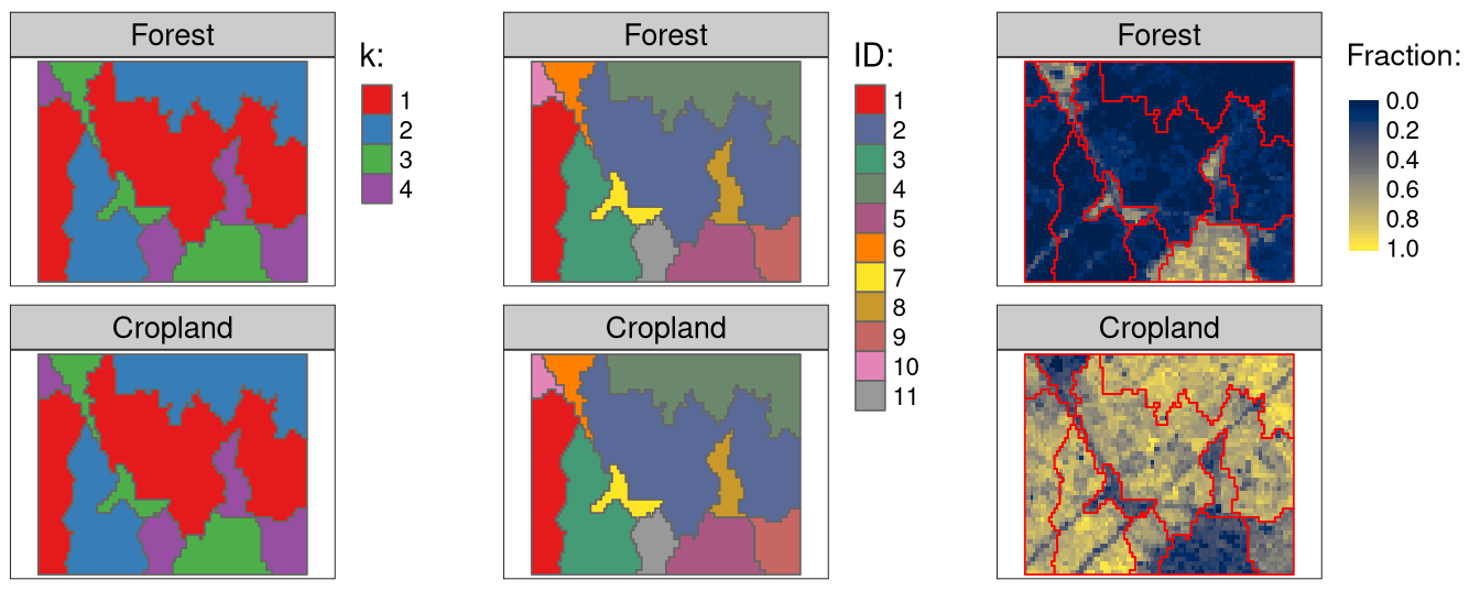
Figure 2 summarized the results. Firstly, we created four clusters using the k-means algorithm (the left panels). You can notice that the first cluster relates to regions with large fractions of forests, while the third cluster has regions with large fractions of croplands. The second and fourth clusters have dominant shares of forests and croplands, respectively. Then each cluster is split into a few regions:

tm1 = tm_shape(flc1[[c(1, 5)]]) +
  tm_raster(legend.show = FALSE) +
  tm_facets(ncol = 1) +
  tm_shape(flc_sc_kmeans) +
  tm_polygons(col = "kmeans", style = "cat", palette = "Set1", title = "k:")
tm2 = tm_shape(flc1[[c(1, 5)]]) +
  tm_raster(legend.show = FALSE) +
  tm_facets(ncol = 1) +
  tm_shape(flc_sc_kmeans2) +
  tm_polygons(col = "kmeans", style = "cat", palette = "Set1", title = "ID:")
tm3 = tm_shape(flc1[[c(1, 5)]]) +
  tm_raster(style = "cont", palette = "cividis", title = "Fraction:") +
  tm_facets(ncol = 1) +
  tm_shape(flc_sc_kmeans2) +
  tm_borders(col = "red")
tmap_arrange(tm1, tm2, tm3)

Figure 2: Regions created with the k-means algorithm on the top of fractions of the forest and cropland classes

SKATER

In this case, an alternative group of methods exists. Instead of using clustering methods, such as k-means, we can use some regionalization methods (they are sometimes referred to as spatial clustering methods).⁵ SKATER (Spatial ’K’luster Analysis by Tree Edge Removal) is a procedure based on a graph representation of the input data. It prunes the graph to its minimum spanning tree (MST) and then iteratively partitions the graph by identifying edges (connections between neighbors) whose removal increases the objective function (between-group dissimilarity) the most. This iterative process stops when a specified number of regions is obtained.

Here, we will use the SKATER procedure as implemented in skater() from the rgeoda package, but we need to start by preparing a few input objects.

The first one is a data frame with the variables of interest for each supercell:

library(rgeoda)

Loading required package: digest

vars = c("Forest", "Shrubland", "Grassland", "Bare.Sparse.vegatation", 
         "Cropland", "Built.up", "Seasonal.inland.water",
         "Permanent.inland.water")
flc_sc_df = st_drop_geometry(flc_sc)[vars]

The second one is an object of class Weight that contains information about neighbors in our data:

queen_w = queen_weights(flc_sc)

The third (optional) object is a vector of distances between values of our supercells. In this case, we will calculate the Jensen-Shannon distance (the same that we used to create our supercells):

weight_dist = philentropy::distance(flc_sc_df, 
                                    method = "jensen-shannon", 
                                    as.dist.obj = TRUE)
weight_dist = as.vector(weight_dist)

Now, we can use the skater() function by providing the expected number of regions (eleven in this case to match the k-means result) and the previously created objects:

skater_results = skater(11, w = queen_w,
                        df = flc_sc_df, rdist = weight_dist)

aaa0x56039dda6d50after gda_skater

Next, we need to add a new column to our data that represents our regions:

flc_sc_skater = flc_sc |> 
  mutate(skater = skater_results$Clusters)

Similarly to the k-means example, we will:

• 1. merge supercells belonging to the same regions:

#1
flc_sc_skater = flc_sc_skater |> 
  group_by(skater) |> 
  summarise() |> 
  st_make_valid()

• 2. add columns with average fractions of each land cover for each region:

#2
names(flc1) = vars
flc_sc_skater_vals = extract(flc1, flc_sc_skater, weights = TRUE) |> 
  group_by(ID) |> 
  summarise(across(all_of(vars), \(x) weighted.mean(x, weight)))
flc_sc_skater = cbind(flc_sc_skater, flc_sc_skater_vals)

Figure 3 shows the SKATER results.

tm1s = tm_shape(flc1[[c(1, 5)]]) +
  tm_raster(legend.show = FALSE) +
  tm_facets(ncol = 1) +
  tm_shape(flc_sc_skater) +
  tm_polygons(col = "skater", style = "cat", palette = "Set1")
tm2s = tm_shape(flc1[[c(1, 5)]]) +
  tm_raster(style = "cont", palette = "cividis", title = "Fraction:") +
  tm_facets(ncol = 1) +
  tm_shape(flc_sc_skater) +
  tm_borders(col = "red")
tmap_arrange(tm1s, tm2s)

Figure 3: Regions created with the SKATER algorithm on the top of fractions of the forest and cropland classes

Quality

The quality of the regionalization results can be evaluated in two main ways: external and internal. The external evaluation compares the obtained regions with, for example, other existing regionalizations. This can be done in R using the sabre package (J. Nowosad and Stepinski 2018).

Here, we will focus on internal evaluation. Internal evaluation checks how well the regions encapsulate similar values and differ from their neighbors. This evaluation can be performed with the two functions of the regional package:

• reg_inhomogeneity() that calculates the internal inhomogeneity of each region (the lower the value, the better)
• reg_isolation() that calculates the isolation of each region from its neighbors (the higher the value, the better)

Let’s start by calculating the inhomogeneity of each region for our two approaches:

vars = c("Forest", "Shrubland", "Grassland", "Bare.Sparse.vegatation", 
         "Cropland", "Built.up", "Seasonal.inland.water", 
         "Permanent.inland.water")
flc_sc_kmeans2$inh = reg_inhomogeneity(flc_sc_kmeans2[vars], flc1, 
                                      dist_fun = "jensen-shannon", 
                                      sample_size = 200)
flc_sc_skater$inh = reg_inhomogeneity(flc_sc_skater[vars], flc1, 
                                      dist_fun = "jensen-shannon", 
                                      sample_size = 200)

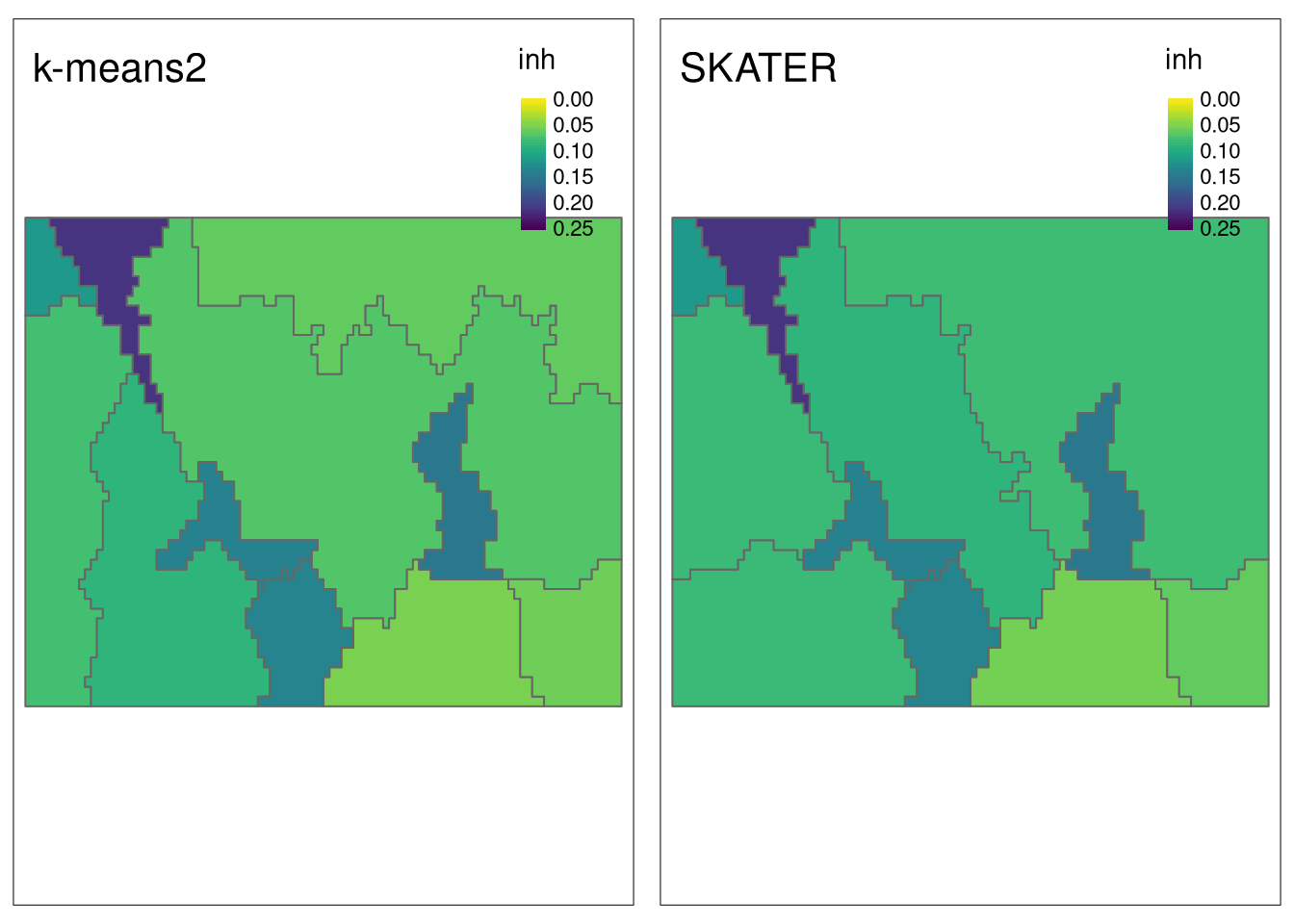
The visual comparison shows that, in general, k-means-based regions have slightly smaller inhomogeneity values.

my_breaks = seq(0, 
                max(flc_sc_kmeans2$inh, flc_sc_skater$inh) + 0.05,
                by = 0.05)
tm_inh2 = tm_shape(flc_sc_kmeans2) + 
  tm_polygons(col = "inh", breaks = my_breaks, style = "cont", palette = "-viridis") +
  tm_layout(title = "k-means2")
tm_inh3 = tm_shape(flc_sc_skater) +
  tm_polygons(col = "inh", breaks = my_breaks, style = "cont", palette = "-viridis") +
  tm_layout(title = "SKATER")
tmap_arrange(tm_inh2, tm_inh3, nrow = 1)

Figure 4: Inhomogeneity of regions created using the k-means and SKATER approaches

This can also be confirmed by calculating area-weighted inhomogeneity, which is a bit smaller for k-means-based regionalization.

area_weighted_inhomogeneity = function(x){
  x$area_km2 = as.numeric(st_area(x)) / 1000000
  round(weighted.mean(x$inh, x$area_km2), 3)
}
area_weighted_inhomogeneity(flc_sc_kmeans2)

[1] 0.08

area_weighted_inhomogeneity(flc_sc_skater)

[1] 0.089

We can also compare how different our regions are from their neighbors with reg_isolation():

flc_sc_kmeans2$iso = reg_isolation(flc_sc_kmeans2[vars], flc1, 
                                      dist_fun = "jensen-shannon", 
                                      sample_size = 200)
flc_sc_skater$iso = reg_isolation(flc_sc_skater[vars], flc1, 
                                      dist_fun = "jensen-shannon", 
                                      sample_size = 200)

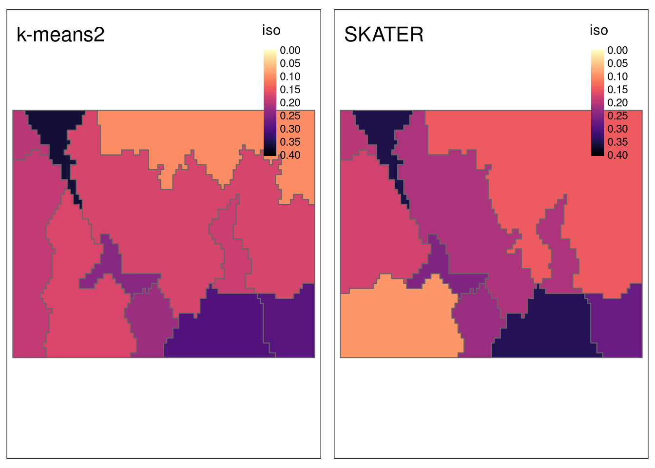
In this case, the maps suggest that SKATER has slightly larger isolation values.

my_breaks2 = seq(0, 
                max(flc_sc_kmeans2$iso, flc_sc_skater$iso) + 0.05,
                by = 0.05)
tm_iso2 = tm_shape(flc_sc_kmeans2) +
  tm_polygons(col = "iso", breaks = my_breaks2, style = "cont", palette = "-magma") +
  tm_layout(title = "k-means2")
tm_iso3 = tm_shape(flc_sc_skater) + 
  tm_polygons(col = "iso", breaks = my_breaks2, style = "cont", palette = "-magma") +
  tm_layout(title = "SKATER")
tmap_arrange(tm_iso2, tm_iso3, nrow = 1)

Figure 5: Isolation of regions created using the k-means and SKATER approaches

This is confirmed by calculating the average isolation for both approaches, which is larger (better) for SKATER:

round(mean(flc_sc_kmeans2$iso), 3)

[1] 0.219

round(mean(flc_sc_skater$iso), 3)

[1] 0.222

Summary

This blog post showed two examples of how to process supercells to create spatially homogeneous regions: one approach used the k-means algorithm, while the other applied the SKATER procedure. It is worth mentioning, however, that many more clustering techniques exist that could be used for this purpose; it includes non-spatial algorithms (e.g., hierarchical clustering) and spatial algorithms (e.g., REDCAP).

The results obtained in this blog post suggested that the k-means approach resulted in (slightly) more homogeneous regions, while regions from the SKATER approach were (also slightly) more isolated from their neighbors. However, you need to remember that the example area was very small and consisted of just a handful of supercells. Our study for a larger area (J. Nowosad, Stepinski, and Iwicki 2022) suggests that SKATER give better results in term of both inhomogeneity and isolation. SKATER (and other spatial clustering methods) should be, in general, preferred over k-means (and other non-spatial clustering methods). They not only result in better regionalizations, but also allow to specify of the output number of regions directly. That being said, the k-means algorithm could also be useful in some cases, especially for large data with hundreds of thousands of supercells (polygons).

If you want to learn more about supercells and regionalizations based on them, we encourage you to try a few entry points. One is the Jakub Nowosad and Stepinski (2022) article that explains the main ideas and applies them to three examples of non-imagery data. You can also see slides from a talk entitled “A method for universal superpixels-based regionalization” that I gave during the FOSS4G 2022 conference at https://jakubnowosad.com/foss4g-2022/. Finally, the package has extensive documentation, including several vignettes, that can be found at https://jakubnowosad.com/supercells/.

References

Aydin, Orhun, Mark. V. Janikas, Renato Martins Assunção, and Ting-Hwan Lee. 2021. “A Quantitative Comparison of Regionalization Methods.” International Journal of Geographical Information Science 35 (11): 2287–2315. https://doi.org/10/gnk4b4.

Nowosad, Jakub, and Tomasz F. Stepinski. 2022. “Extended SLIC Superpixels Algorithm for Applications to Non-Imagery Geospatial Rasters.” International Journal of Applied Earth Observation and Geoinformation 112 (August): 102935. https://doi.org/10.1016/j.jag.2022.102935.

Nowosad, J., and T. F. Stepinski. 2018. “Spatial Association Between Regionalizations Using the Information-Theoretical V -Measure.” International Journal of Geographical Information Science 32 (12): 2386–2401. https://doi.org/10/gf283f.

Nowosad, J., T. F. Stepinski, and M. Iwicki. 2022. “A method for universal supercells-based regionalization (preliminary results).” The International Archives of the Photogrammetry, Remote Sensing and Spatial Information Sciences XLVIII-4/W1-2022 (August): 337–44. https://doi.org/10.5194/isprs-archives-XLVIII-4-W1-2022-337-2022.

Footnotes

1. There are several approaches for deciding the number of clusters. Some are based on prior knowledge and some use various methods to suggest an optimal k number (e.g., Elbow method).

2. Try plot(flc_sc_kmeans["kmeans"])

3. Additionally, we used st_make_valid() to make sure that our result has valid geometries.

4. Area-weighted mean, to be precise.

5. Read Aydin et al. (2021) to see a comparison of regionalizations methods.