Finding the most unique land cover spatial pattern

Spatial signatures represent spatial patterns of land cover in a given area. Thus, they can be used to search for areas with similar spatial patterns to a query region or to quantify changes in spatial patterns. The approaches above are implemented as lsp_search() and lsp_compare() functions of the motif R package, respectively.

At the same time, it is possible to create other, more customized workflows. Here, I will show how to compare spatial patterns of two different areas and find the most unique land cover spatial pattern in the process.

Spatial data

To reproduce the calculations in the following post, you need to download all of the relevant datasets using the code below:

library(osfr)
dir.create("data")
osf_retrieve_node("xykzv") |>
        osf_ls_files(n_max = Inf) |>
        osf_download(path = "data",
                     conflicts = "skip")

You should also attach the following packages:

library(sf)
library(terra)
library(motif)
library(dplyr)
library(readr)
library(cluster)

Land cover in Africa

The data/land_cover.tif contains land cover data for Africa. It is a categorical raster of the 300-meter resolution that can be read into R using the rast() function.

lc = rast("data/land_cover.tif")

Additionally, the data/lc_palette.csv file contains information about the labels and colors of each land cover category.

lc_palette_df = read.csv("data/lc_palette.csv")

We will use this file to integrate labels and colors into the raster object:

levels(lc) = lc_palette_df[c("value", "label")]
coltab(lc) = lc_palette_df[c("value", "color")]
plot(lc)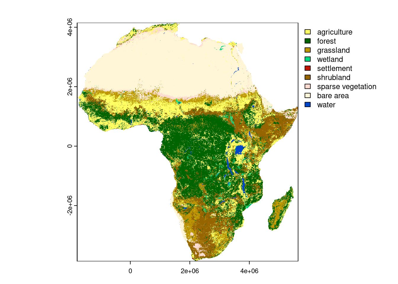

Comparing spatial patterns of two areas

First, we need to define the areas for which we want to compare spatial patterns. For the example purpose, we use two African countries: Cameroon and Congo. We can download their areas using the rnaturalearth package, and use them to crop the lc raster object to their borders:

library(rnaturalearth)
# download
cameroon = ne_countries(country = "Cameroon", returnclass = "sf") |>
  select(name) |>
  st_transform(crs = st_crs(lc))
congo = ne_countries(country = "Republic of the Congo", returnclass = "sf") |>
  select(name) |>
  st_transform(crs = st_crs(lc))
# crop
lc_cameroon = crop(lc, cameroon, mask = TRUE)
lc_congo = crop(lc, congo, mask = TRUE)
# plot
plot(lc_cameroon)
plot(lc_congo)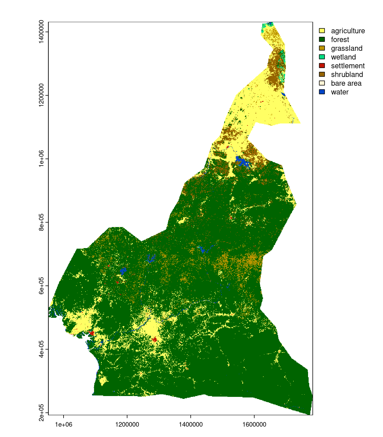

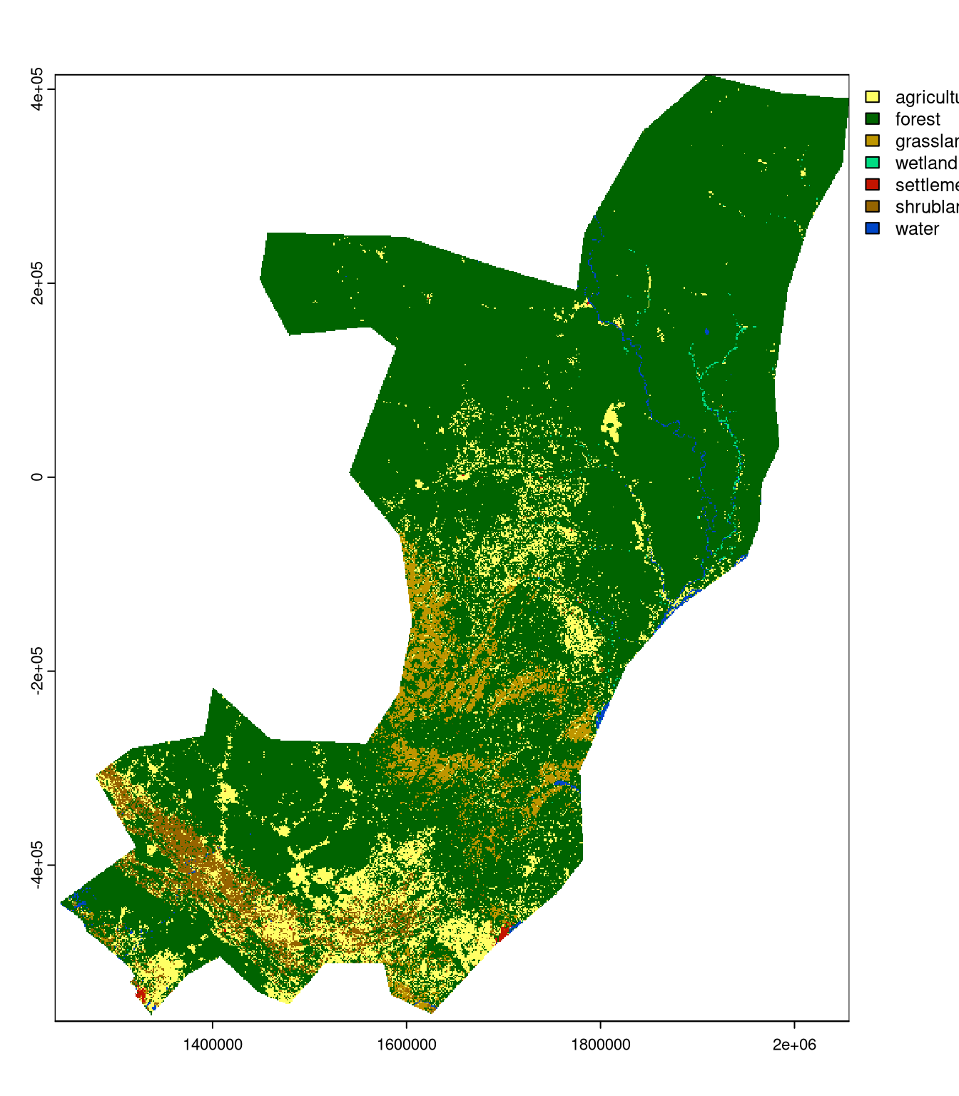
Both countries have similar shares of land cover categories, with the domination of forests and some agricultural and grassland areas, as we can see by calculating their "composition" signatures.

lc_cameroon_composition = lsp_signature(lc_cameroon, type = "composition", classes = 1:9)
lc_congo_composition = lsp_signature(lc_congo, type = "composition", classes = 1:9)
round(lc_cameroon_composition$signature[[1]], 2)

        1    2    3 4 5    6 7 8    9
[1,] 0.15 0.77 0.03 0 0 0.04 0 0 0.01

round(lc_congo_composition$signature[[1]], 2)

       1    2    3 4 5    6 7 8 9
[1,] 0.1 0.82 0.04 0 0 0.03 0 0 0

We can also look at their spatial patterns (both composition and configuration) by calculating the "cove" signature.

lc_cameroon_cove = lsp_signature(lc_cameroon, type = "cove", classes = 1:9)
lc_congo_cove = lsp_signature(lc_congo, type = "cove", classes = 1:9)

Next, these signatures can be compared using dissimilarity measures. The philentropy package provides a wide range of such measures, including the Jensen-Shannon divergence. Here, we use this measure to calculate the dissimilarity between the spatial patterns (as represented with "cove") of Cameroon and Congo.

library(philentropy)
dist_cove = dist_one_one(lc_cameroon_cove$signature[[1]], 
                         lc_congo_cove$signature[[1]], 
                         method = "jensen-shannon")
dist_cove

[1] 0.008919291

This value is small (approximately 0.009), which means that, in general, Cameroon’s and Congo’s spatial patterns are fairly similar.

Comparing local spatial patterns

We can also look at the local spatial patterns of Cameroon and Congo, here on a scale of 100 by 100 cells (i.e., 30 by 30 km):

lc_cameroon_cove100 = lsp_signature(lc_cameroon, type = "cove",
                                    window = 100, classes = 1:9)
lc_congo_cove100 = lsp_signature(lc_congo, type = "cove", 
                                 window = 100, classes = 1:9)

To compare these signatures, we can calculate the Jensen-Shannon divergence for each pair of signatures in both datasets. This can be done using the dist_many_many() function from the philentropy package, which expects two matrices as input.

lc_cameroon_cove100_mat = do.call(rbind, lc_cameroon_cove100$signature)
lc_congo_cove100_mat = do.call(rbind, lc_congo_cove100$signature)
dist_cove_100 = dist_many_many(lc_cameroon_cove100_mat, 
                               lc_congo_cove100_mat, 
                               method = "jensen-shannon")

The result is a matrix with the Jensen-Shannon divergence between each pair of areas in both countries, in which rows represent areas in Cameroon and columns represent areas in Congo. Lower values indicate more similar spatial patterns, while higher values indicate more dissimilar spatial patterns. This matrix shows that there are some areas with similar spatial patterns in both countries, and some are even identical (given the source data scale/resolution and scope/number and variety of categories):

summary(c(dist_cove_100))

   Min. 1st Qu.  Median    Mean 3rd Qu.    Max. 
0.00000 0.03228 0.08722 0.16375 0.22835 0.69315 

Identifiers of the identical areas can be found using the which() function. For example, area 341 in Cameroon and area 4 in Congo have the same spatial pattern:

head(which(dist_cove_100 == 0, arr.ind = TRUE))

     row col
[1,] 341   4
[2,] 418   4
[3,] 423   4
[4,] 440   4
[5,] 462   4
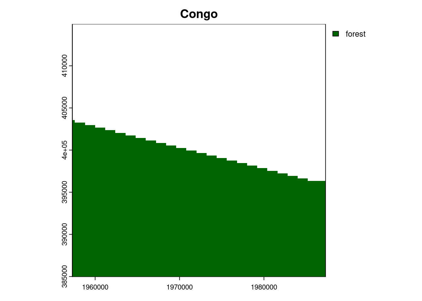
[6,] 477   4

We can add spatial information to the lc_cameroon_cove100 and lc_congo_cove100 objects using the lsp_add_sf() function. Then, we are able to visualize these areas by cropping the land cover data using the new objects. In this case, both areas are fully covered by forest (although the second one is located at the border, and thus contains some NA values).

lc_cameroon_cove100_sf = lsp_add_sf(lc_cameroon_cove100)
lc_congo_cove100_sf = lsp_add_sf(lc_congo_cove100)
plot(crop(lc_cameroon, lc_cameroon_cove100_sf[341, ]), main = "Cameroon")
plot(crop(lc_congo, lc_congo_cove100_sf[4, ]), main = "Congo")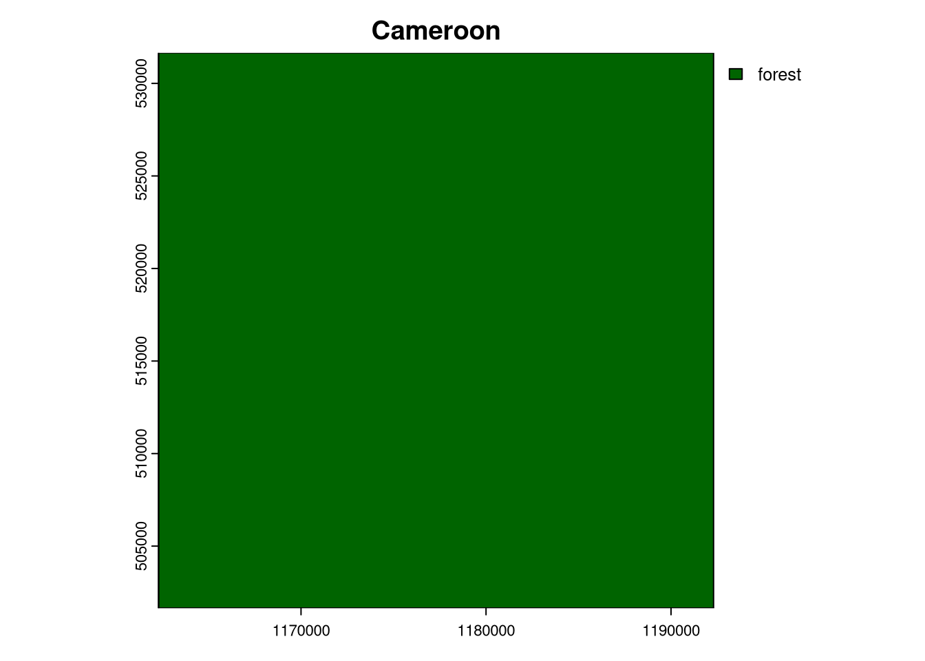

Grouping areas with similar local spatial patterns

We can group areas with similar spatial patterns of land cover using the pam() function from the cluster package. For this example, we will divide the areas into six groups.

my_pam = pam(rbind(lc_cameroon_cove100_mat, lc_congo_cove100_mat), 6)

Next, we can add the clustering results to the spatial object by naming both existing sf objects, combining them into one, and adding the clustering results as a new column.

lc_cameroon_cove100_sf$name = "Cameroon"
lc_congo_cove100_sf$name = "Congo"
lc_cove100_sf = rbind(lc_cameroon_cove100_sf, lc_congo_cove100_sf)
lc_cove100_sf$k = as.factor(my_pam$clustering)

Visualization of the results is shown below:

plot(subset(lc_cove100_sf, name == "Cameroon")["k"], pal = palette.colors, main = "Cameroon")
plot(subset(lc_cove100_sf, name == "Congo")["k"],  pal = palette.colors, main = "Congo")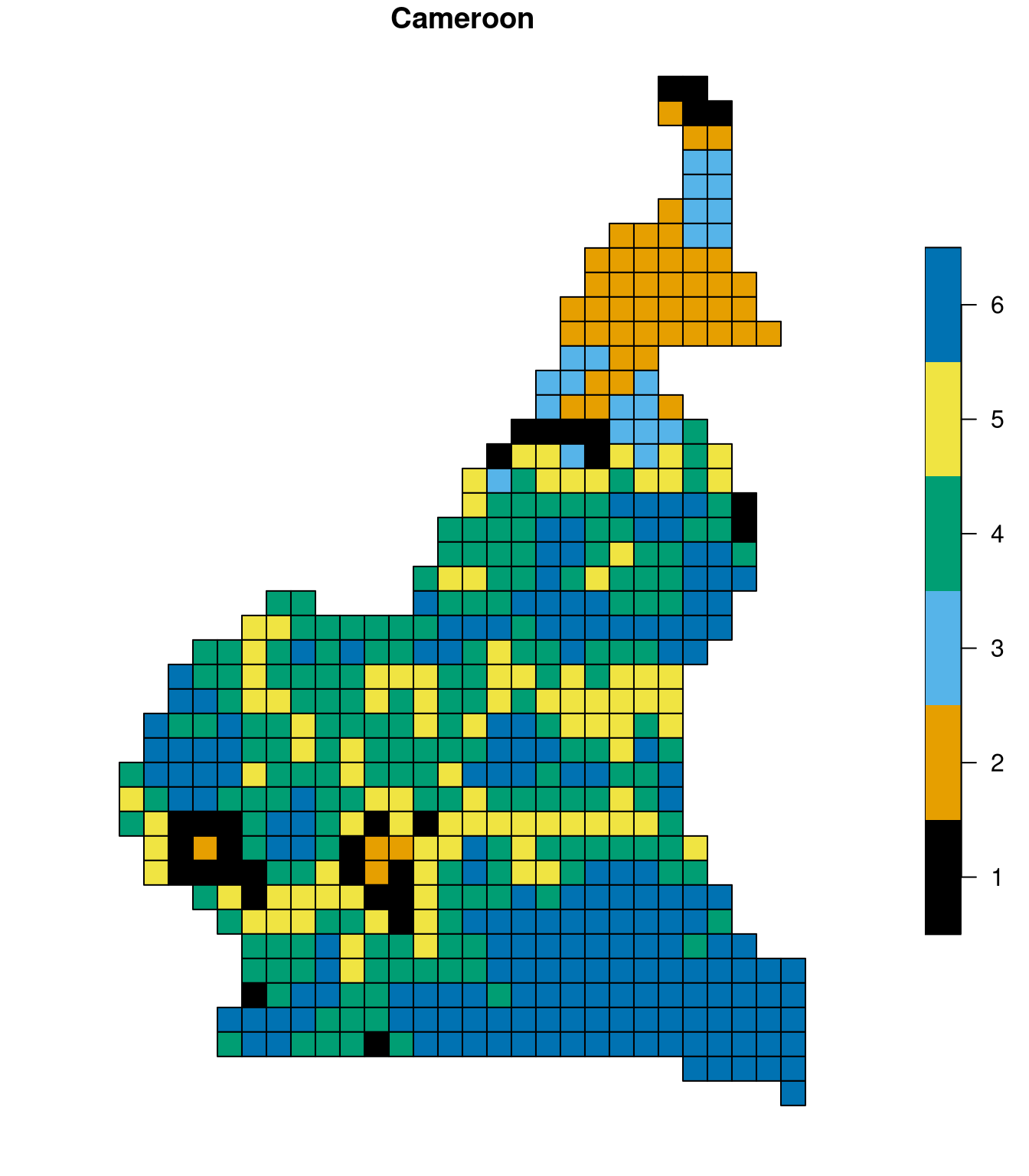

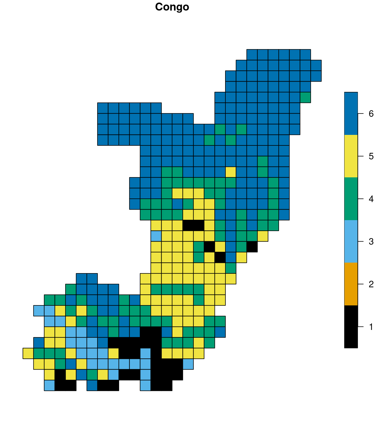
You may quickly notice that the sixth and fifth clusters exist prominently in both countries. On the other hand, cluster 2 only exists in Cameroon.

We can look at each cluster representative by subsetting the lc_cove100_sf object using the id.med column from the my_pam object.

lc_cove100_sf_subset = lc_cove100_sf[my_pam$id.med, ]
for (i in seq_len(nrow(lc_cove100_sf_subset))){
  plot(crop(lc, lc_cove100_sf_subset[i, ]), main = i)
}

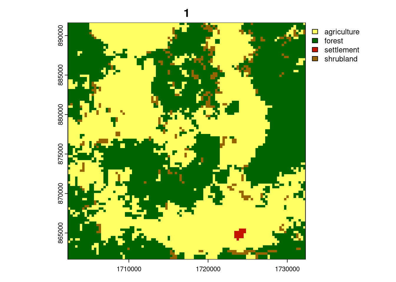
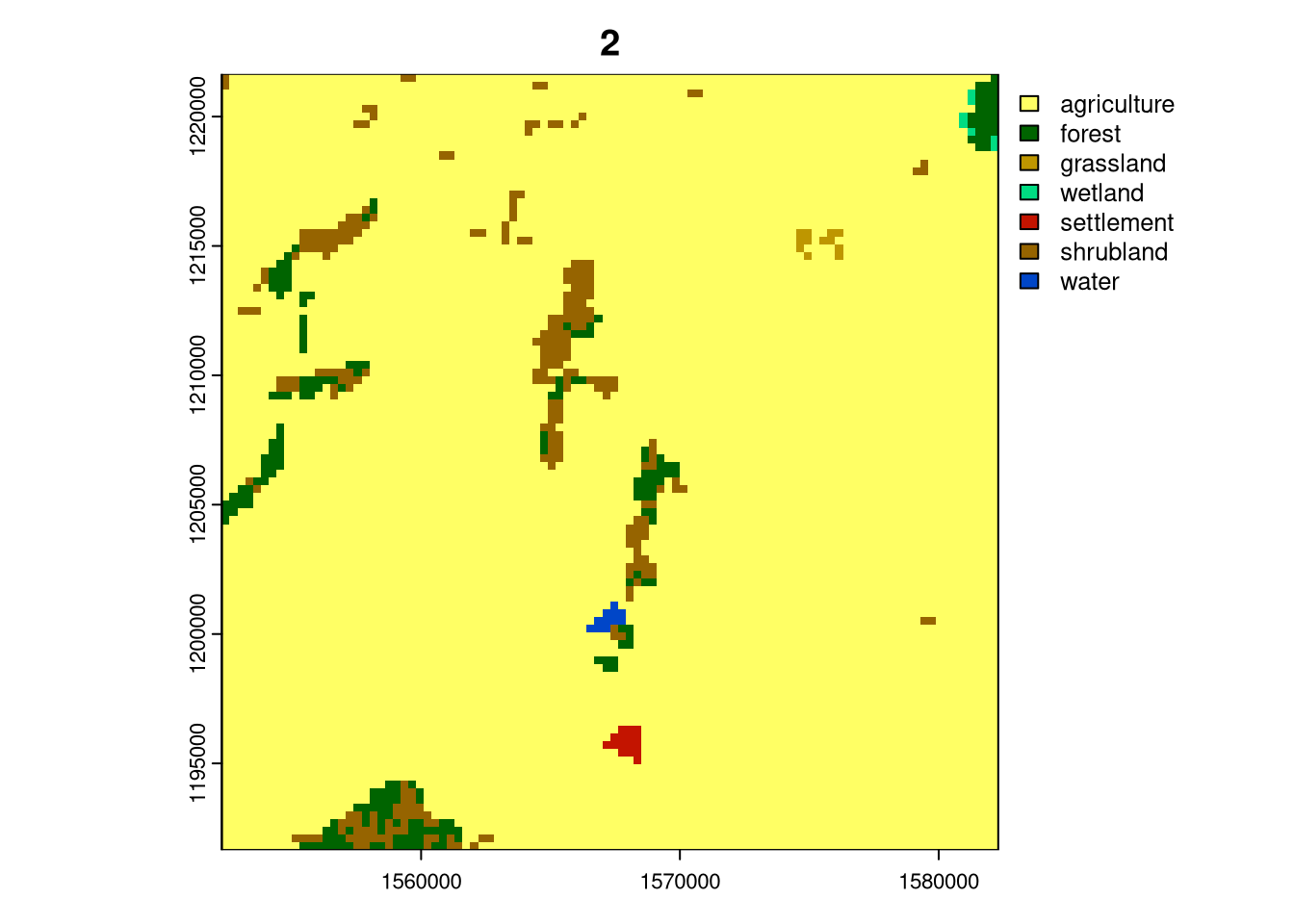
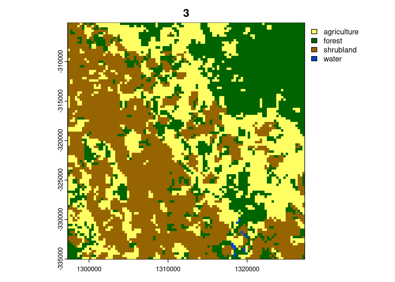
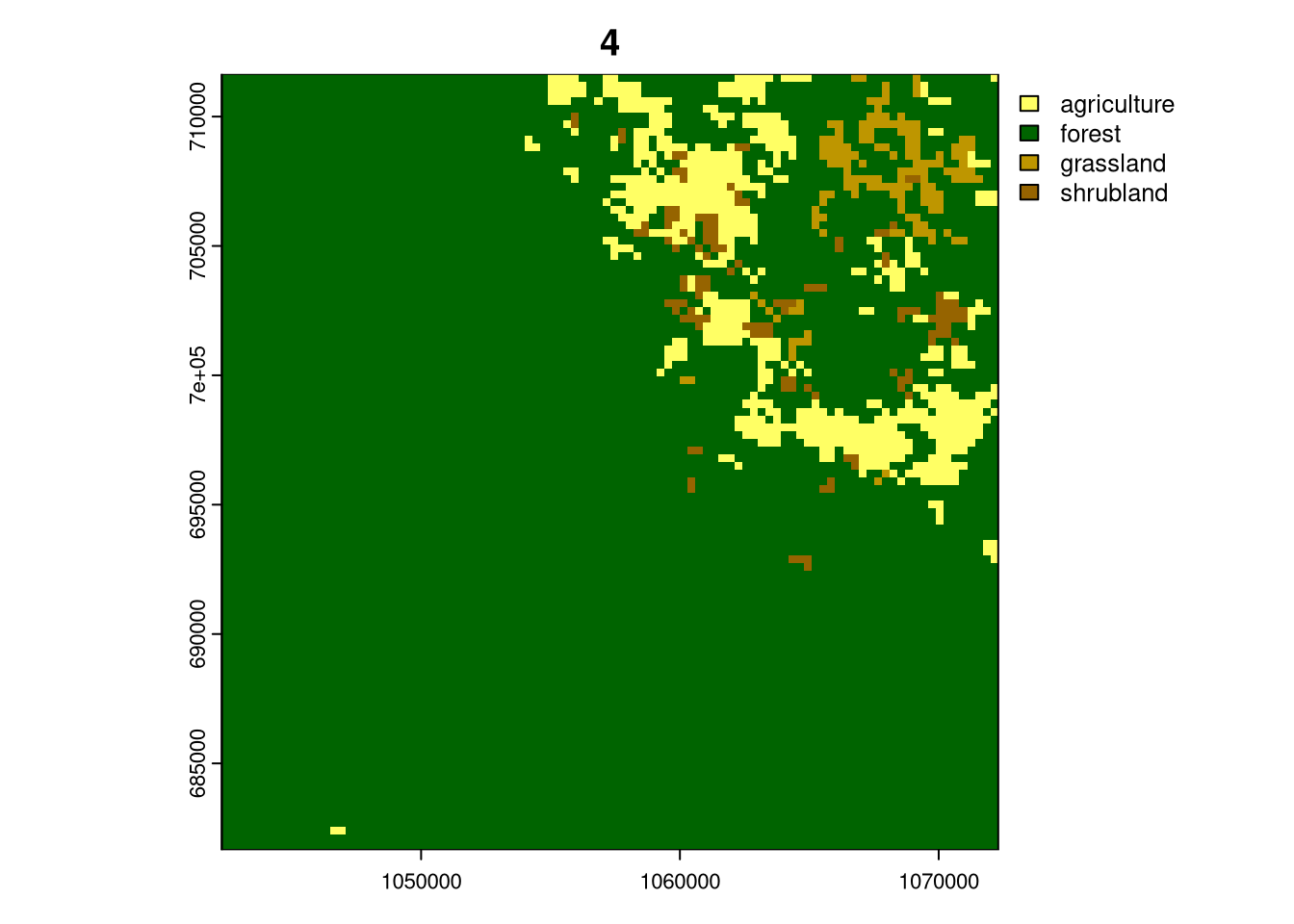
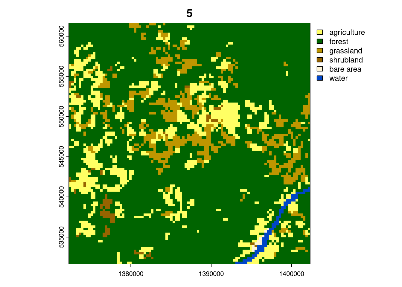
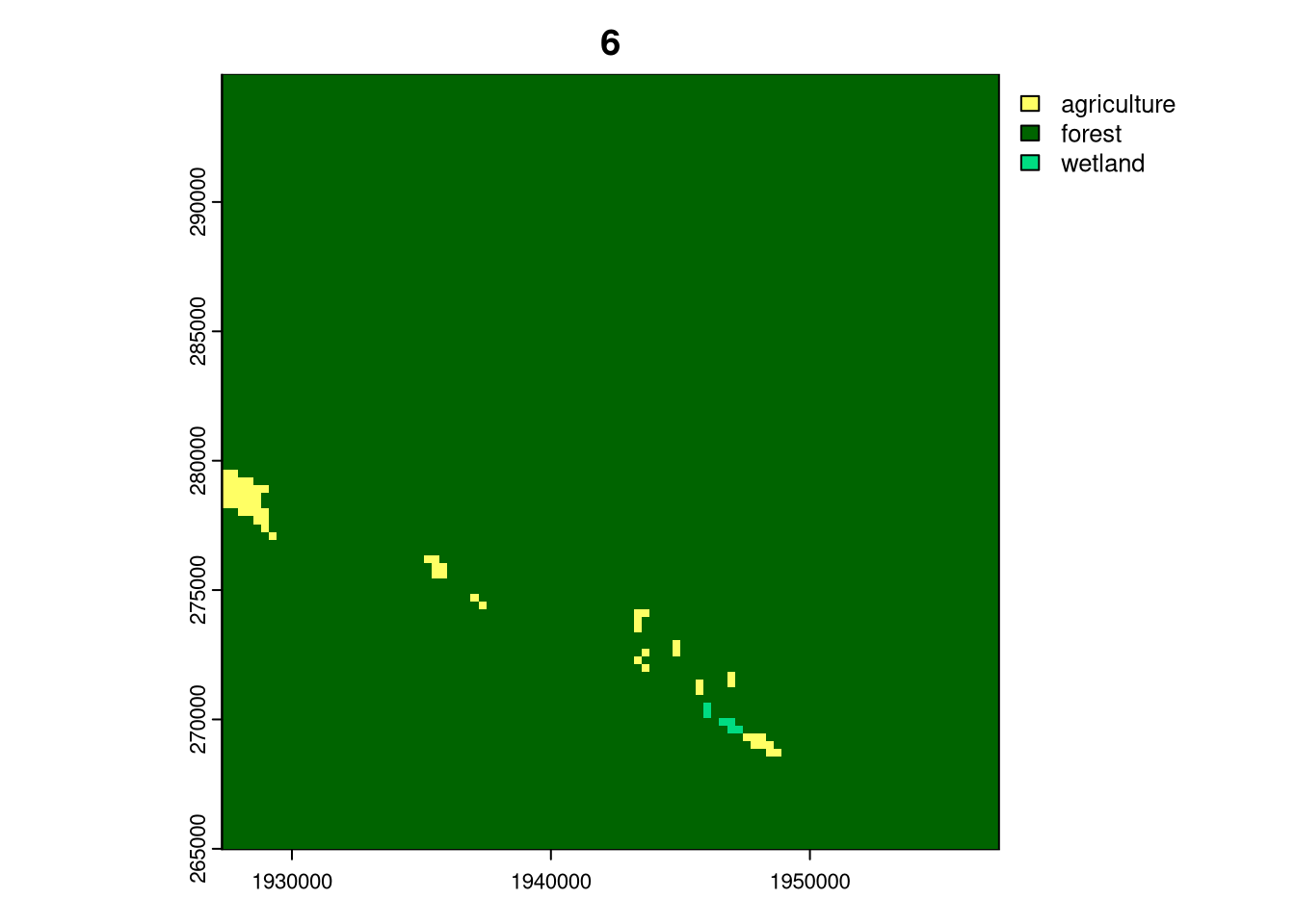
Cluster 6 represents forest areas, and cluster 4 consists of areas predominantly covered by forests and some agricultural and grassland areas. Cluster 5 is represented by forest, but with a substantial share of agriculture and grasslands and cluster 1 is a mix of highly aggregated agriculture and forest. Cluster 3 are areas with a large share of shrublands, agricultural and forest areas. Finally, cluster 2, which only exists in Cameroon, represents large (30 by 30 km) areas of agriculture.

Finding the most unique land cover spatial pattern

The dist_cove_100 object contains the Jensen-Shannon divergence between each pair of areas in both countries, where rows represent areas in Cameroon and columns represent areas in Congo. Usually, it may be used to find the most similar areas (areas with the smallest divergence), but here, we will look for the most unique areas.

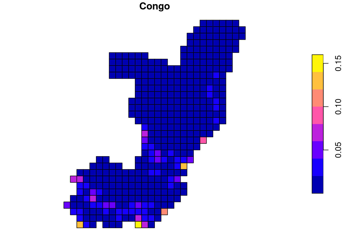
This can be done in two steps. First, we need to calculate the smallest value in each row and column, which can be done using the apply() function. This allows us to find what is the smallest divergence between each area in Cameroon and Congo; in other words, how dissimilar is an area in one country to the most similar area in the other country.

lc_cameroon_cove100_sf$min_dist = apply(dist_cove_100, 1, min)
plot(lc_cameroon_cove100_sf["min_dist"], main = "Cameroon")
lc_congo_cove100_sf$min_dist = apply(dist_cove_100, 2, min)
plot(lc_congo_cove100_sf["min_dist"], main = "Congo")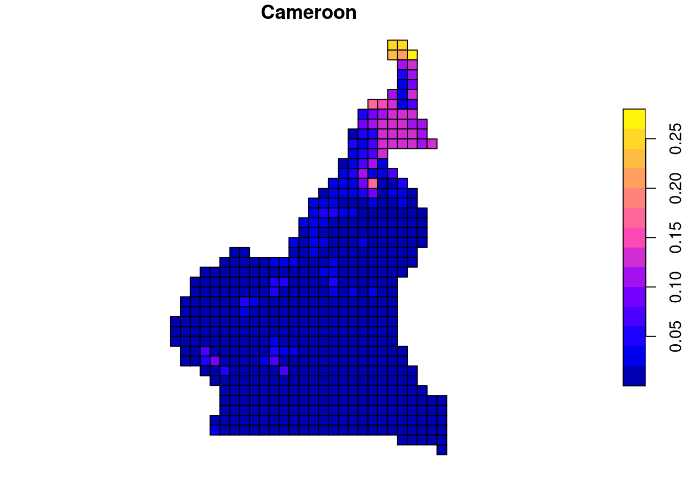

Second, we can find the area with the largest value in the lc_cameroon_cove100_sf$min_dist column, which is the most unique area in Cameroon, and the area with the largest value in lc_congo_cove100_sf$min_dist, which is the most unique area in Congo. In other words, these areas are the most dissimilar to any area in the other country.

most_unique_cameroon = lc_cameroon_cove100_sf[which.max(lc_cameroon_cove100_sf$min_dist), ]
plot(crop(lc_cameroon, most_unique_cameroon), main = "Cameroon")
most_unique_congo = lc_congo_cove100_sf[which.max(lc_congo_cove100_sf$min_dist), ]
plot(crop(lc_congo, most_unique_congo), main = "Congo")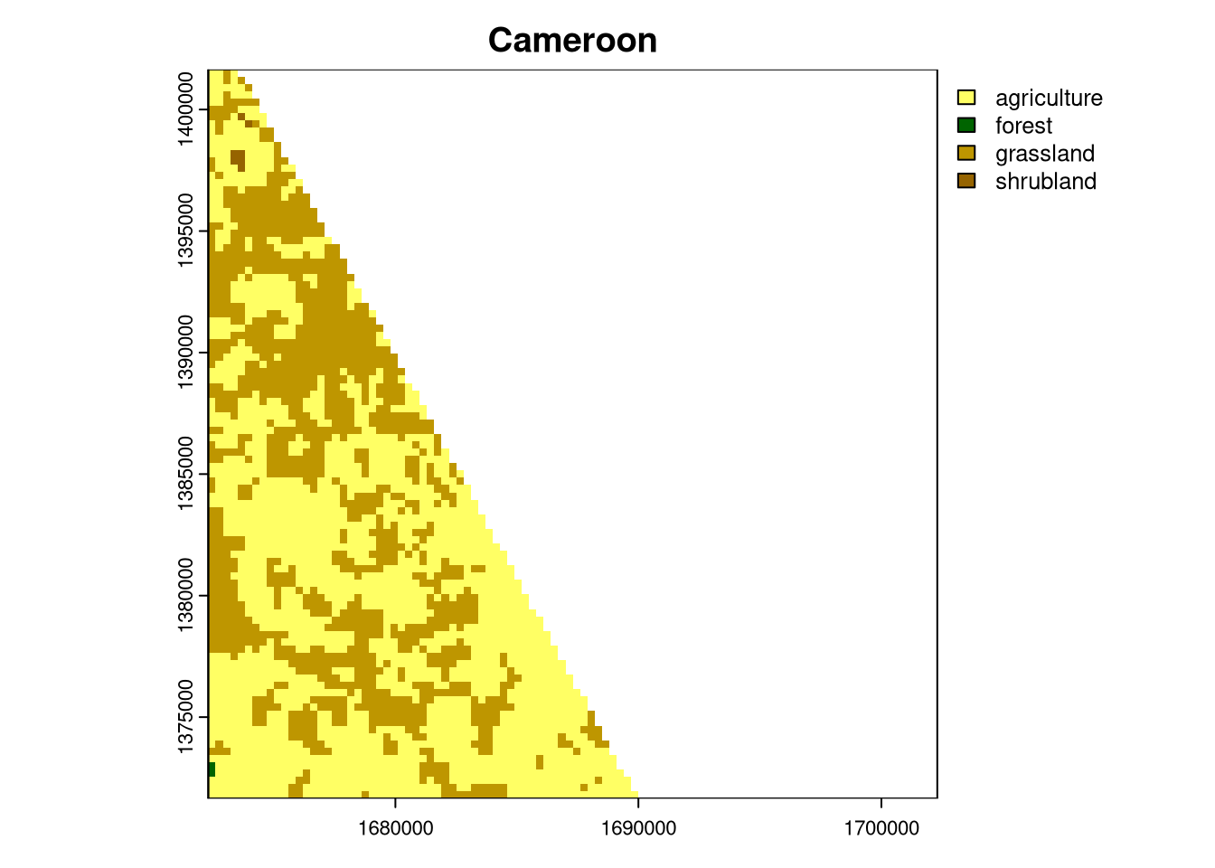

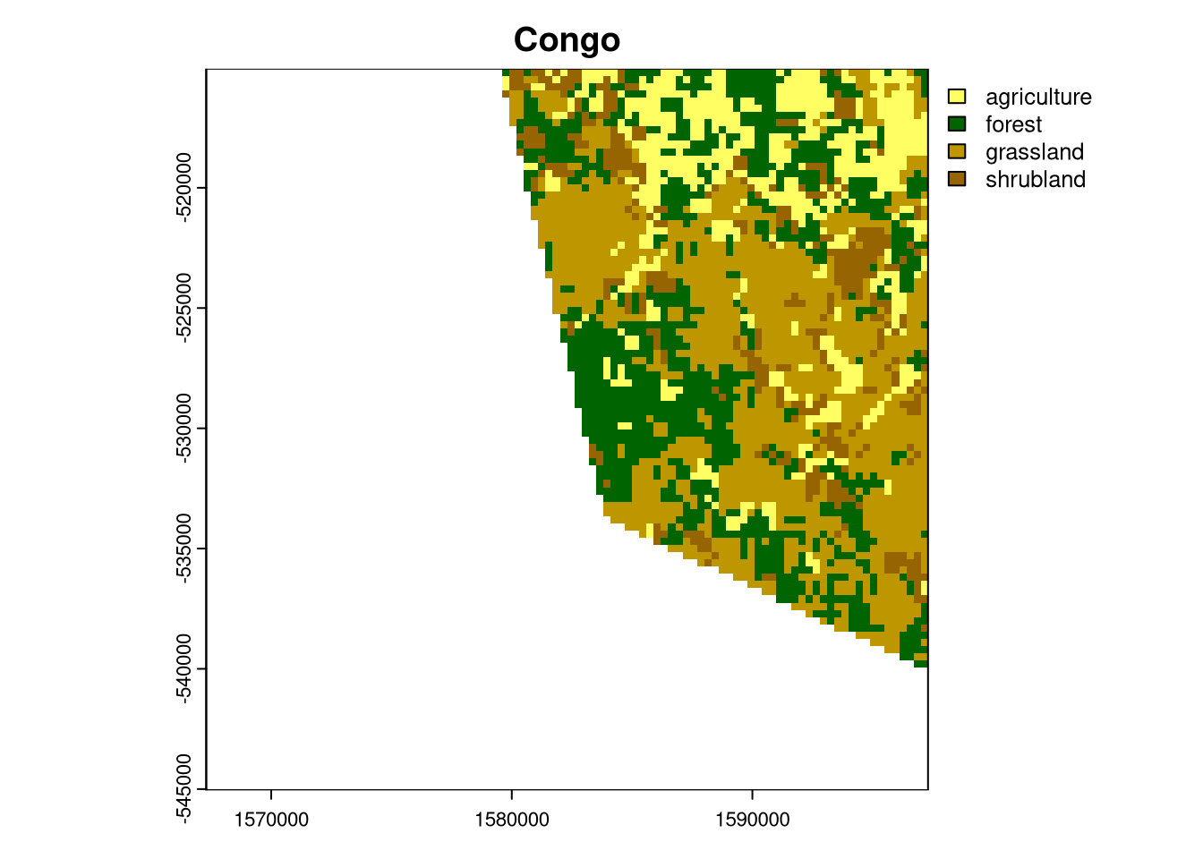
In the case of Cameroon, such an area is a mosaic of agriculture and grasslands; for Congo, it is a complex area with grasslands, agriculture, forest, and some shrublands. Interestingly, both areas are located at the border of the countries.¹

Summary

In this post, we have seen how to compare spatial patterns of land cover in two different areas. It also showed how to find the most unique land cover spatial pattern (try to find the most unique area in your country as compared to the rest of the world!) This approach can be used to find areas with unique spatial land cover patterns or any other categorical rasters. To learn more about the motif package, see the other blog posts in the “motif” category.

Footnotes

1. You could change the threshold parameter in lsp_signature() to 0 to only include areas completely inside the countries’ borders.