Simulating spatial patterns with the spatial kinetic Ising model

A two-dimensional Ising model is an idealized physical system that consists of a lattice of binary variables (magnetic spins) that can be in one of two states: up or down. Each spin’s state is influenced by its neighbors: the more neighbors in the same state, the more likely the spin will be in the same state. Thus, the change in the state of a spin impacts the state of its neighbors, which in turn affects the state of their neighbors, and so on. It is a simple model that can be used in physics to study, for example, phase transitions given by the temperature of the system.

The above idea can be, in principle, applied to other two-dimensional systems, such as geographical (spatial) data. For example, we can think of a binary spatial raster as a two-dimensional system, where each cell can have one of two states: -1 or 1. These numbers can represent, for example, two land cover categories: forest and non-forest. Next, we can introduce two parameters influencing the state of each cell: B and J. B is an external pressure: it tries to align cells’ values with its sign: are we more likely to have more -1 or 1 values? J is a strength of the local autocorrelation tendency—it tries to align signs of neighboring cells: are we more likely to have more cells of the same value in the neighborhood? The spatial kinetic Ising model is a simulation of such a system, where each cell is given an opportunity to flip its value (1 to -1 or -1 to 1). The probability of a flip depends on the value of the cell, the values of its four neighbors (top, left, bottom, and right), and the values of B and J.

This blog post shows how to use the spatial kinetic Ising model to simulate the change in the spatial pattern of a binary raster using the spatialising R package. The package is available on GitHub at https://github.com/Nowosad/spatialising/.

Setup

To reproduce the calculations in the following post, you need to attach the following packages:

library(terra)
library(spatialising)
library(ggplot2)

Data preparation

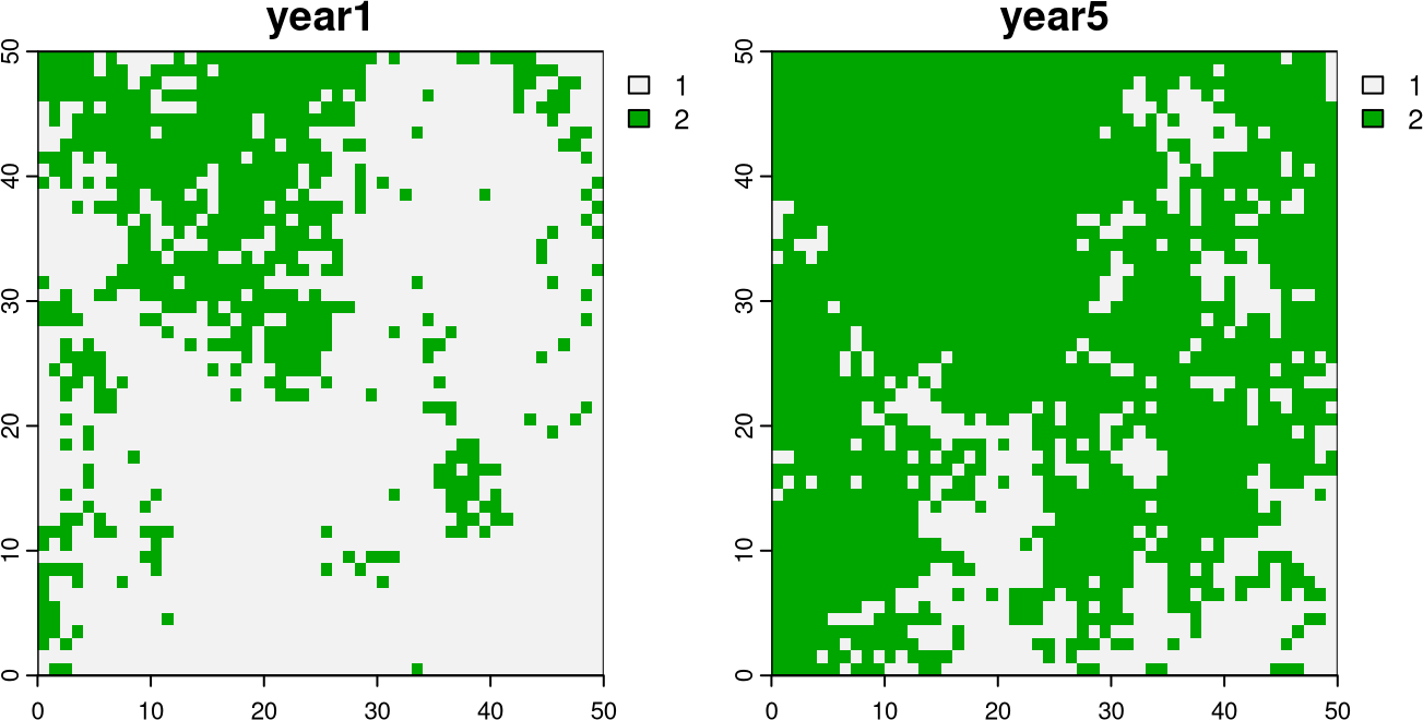
The twomaps.tif file contains two maps of the same area, but for different years. The first map represents the year 1, and the second map represents the year 5. Both of them have only two values: 1 for non-forest and 2 for forest:

twomaps = rast("/vsicurl/https://github.com/Nowosad/bp-data/raw/main/spatialising-bp/twomaps.tif")
map1 = twomaps[[1]]
map2 = twomaps[[2]]
plot(c(map1, map2))

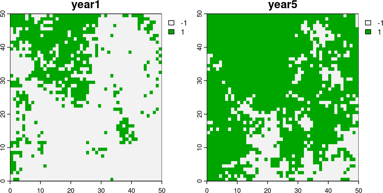
The spatial kinetic Ising model requires binary raster data with just two values: -1 and 1. Thus, the first step in our case is to reclassify the original binary (1, 2) map into new (-1, 1) values. This can be done with the classify() function from the terra package.¹ Here, we replace the 1 value with -1 and the 2 value with 1:

rcl = matrix(c(1, -1, 2, 1), byrow = TRUE, ncol = 2)
map1 = classify(map1, rcl)
map2 = classify(map2, rcl)
plot(c(map1, map2))

Running the spatial kinetic Ising model

Now, our data is ready for use in the spatialising package. Its main function is kinetic_ising(), which simulates the spatial kinetic Ising model. It requires the input raster (x), the strength of the external pressure (B), the strength of the local autocorrelation tendency (J), and also has some optional arguments, such as the number of updates.

Our goal is to simulate the change in the spatial pattern of the first map (map1) to make it similar to the second map (map2). The code below simulates the spatial kinetic Ising model for the first map (map1) with the value of B of 0.3 (meaning that the external pressure is toward increased forest cover) and the value of J of 0.7 (meaning that the local autocorrelation tendency is strong). We also set the number of updates to 4, which means that it will create four simulations (rasters), each of which will be based on the previous one.²

sim1 = kinetic_ising(map1, B = 0.3, J = 0.7, updates = 4)
plot(sim1, nr = 1)

The result consists of four simulated rasters, which are stored in the sim1 object. Each of them represents successive simulations of the spatial kinetic Ising model.

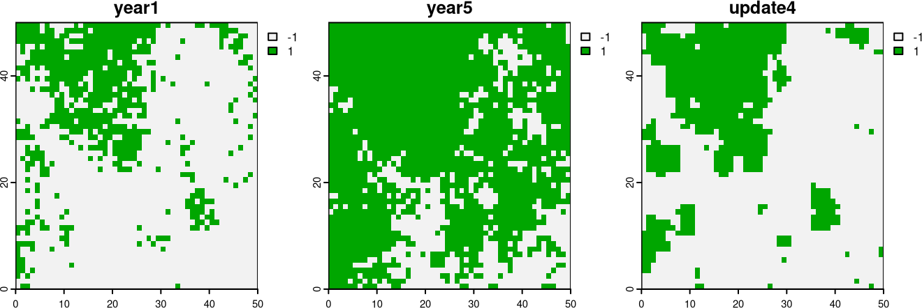
We can also compare the final simulation (sim1[[4]]) with the first (map1) and the second map (map2).

plot(c(map1, map2, sim1[[4]]), nr = 1)

Compared to the first map, the last simulation has slightly more forest cover, which is in line with the provided external pressure (B) toward increased forest cover. The forest category also tends to be spatially clustered, which is in line with the set local autocorrelation tendency (J). On the other hand, the simulation is still quite different from the second map (map2), possibly indicating that we should increase the value of B to make the simulation more like the second map.

Metrics of spatial patterns

The spatialising package also provides two functions to calculate metrics of spatial patterns of binary rasters: composition_index() and texture_index(). The composition imbalance index (composition_index()) is a sum of cell’s values over the entire site divided by the number of cells in the site. It has a range from -1 (site completely dominated by the -1 values) to 1 (site completely dominated by the 1 values). The value of 0 indicates that the site is equally divided between the two values.

composition_index(c(map1, map2, sim1[[4]]))

[1] -0.5000  0.5000 -0.4184

In our case, map1 has a dominance of the -1 values, map2 has a dominance of the 1 values, and sim1[[4]] has a dominance of the -1 values, but it is less pronounced than in map1.

The texture index (texture_index()) is a measure of the spatial autocorrelation of the values of a raster. Its value is between 0 (fine texture), and 1 (coarse texture).

texture_index(c(map1, map2, sim1[[4]]))

[1] 0.6477551 0.6216327 0.8387755

In our examples, map1 and map2 have a rather similar texture, while sim1[[4]] has a slightly coarser texture (its values have stronger spatial autocorrelation).

Spatial kinetic Ising model explained

How does the spatial kinetic Ising model work? The simulation starts with the input binary (-1, 1) raster and proceeds with one randomly selected cell at a time. The selected cell is given an opportunity to flip its value (1 to -1 or -1 to 1). The probability of a flip depends on the value of the cell and the values of its four neighbors (top, left, bottom, and right). It also depends on the values of B and J. B (positive or negative) is an external pressure: it tries to align cells’ values with its sign. J (always positive) is a strength of the local autocorrelation tendency: it tries to align signs of neighboring cells.

We can also control the model using a few additional arguments. The iter argument controls the number of iterations—how many times the flip of a cell value is attempted before a new simulated raster is returned. By default, its value equals to the number of cells in the input raster. Next, updates controls the number of simulated rasters returned—each of which is based on the previous one. The inertia parameter (0, by default), when positive makes it less likely for a cell of -1 to change its value to 1 when surrounded by other -1 cells. As the effect, it minimizes the possibility of a “salt and pepper” effect, where cells of different values are mixed together. The last important argument is rule, which controls how the probability of a flip is calculated: either using the "glauber" (default) or "metropolis" rule.

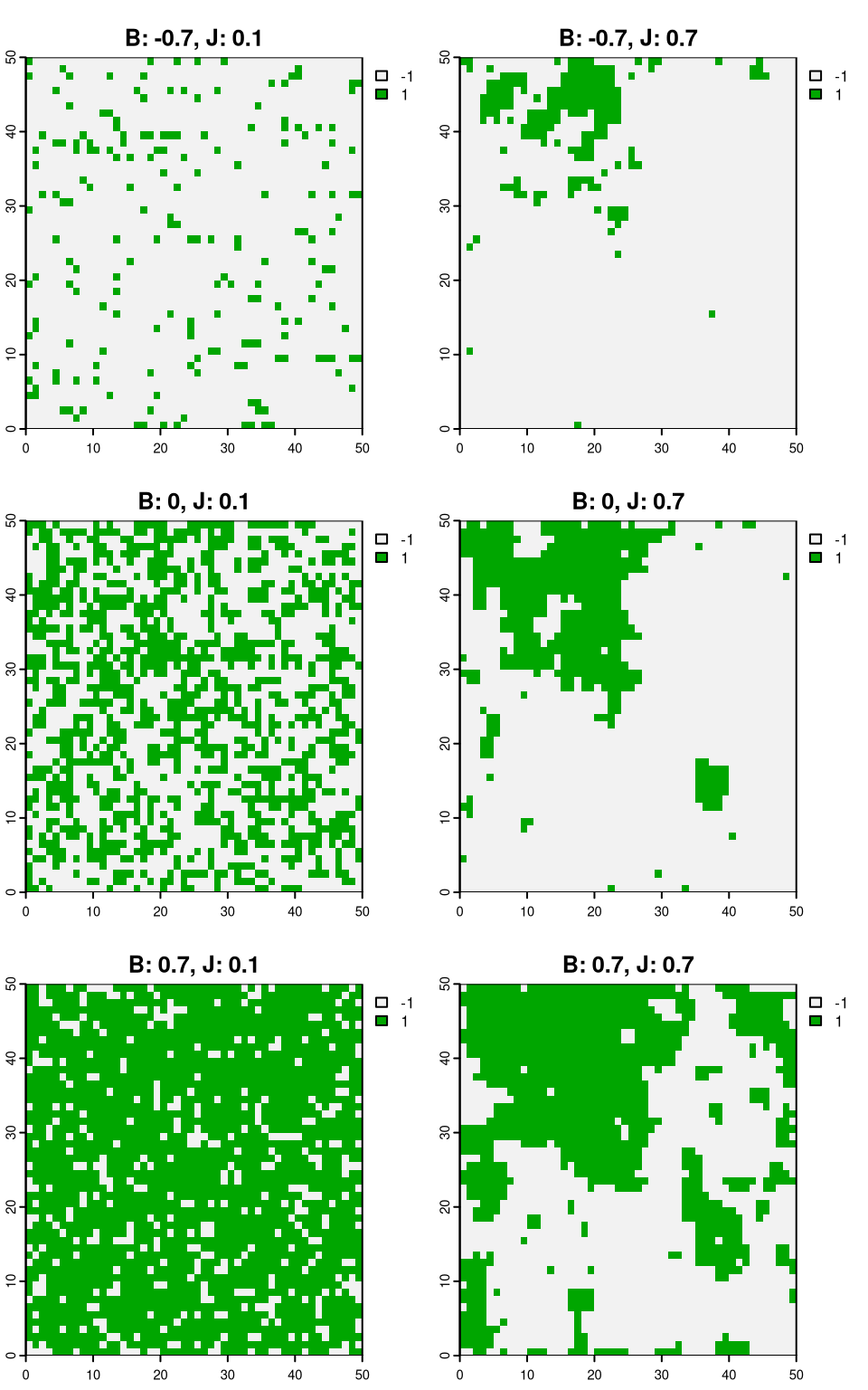
The code below compares the results of the spatial kinetic Ising model for different values of B and J.

sim2 = kinetic_ising(map1, B = -0.7, J = 0.1, updates = 4, inertia = 1)
sim3 = kinetic_ising(map1, B = -0.7, J = 0.7, updates = 4, inertia = 1)
sim4 = kinetic_ising(map1, B = 0, J = 0.1, updates = 4, inertia = 1)
sim5 = kinetic_ising(map1, B = 0, J = 0.7, updates = 4, inertia = 1)
sim6 = kinetic_ising(map1, B = 0.7, J = 0.1, updates = 4, inertia = 1)
sim7 = kinetic_ising(map1, B = 0.7, J = 0.7, updates = 4, inertia = 1)
all_sims = c(sim2[[4]], sim3[[4]], sim4[[4]], sim5[[4]], sim6[[4]], sim7[[4]])
names(all_sims) = c("B: -0.7, J: 0.1", "B: -0.7, J: 0.7", "B: 0, J: 0.1", 
                    "B: 0, J: 0.7", "B: 0.7, J: 0.1", "B: 0.7, J: 0.7")
plot(all_sims, nc = 2)

The top row shows the results for B values equal to -0.7, the middle row shows the results for B values equal to 0, and the bottom row shows the results for B values equal to 0.7. The left column shows the results of the spatial kinetic Ising model for values of J equal to 0.1, while the right column shows the results for values of J equal to 0.7.

Quick visual comparison underlines that both parameters have a strong effect on the results of the spatial kinetic Ising model. Negative values of B tend to decrease the forest cover, while positive values of B tend to increase the forest cover. The effect of J is, on the other hand, more related to the configuration of the values, with lower values of J leading to more dispersed values, and higher values of J leading to more clustered values.

Summary

This blog post showed how to use the spatialising package to simulate the spatial kinetic Ising model, how selected parameters influence the results, and how to calculate metrics of spatial patterns. However, it leaves one important question unanswered: how do you find the best values of B and J to make the simulation more like the second map? That is the topic of the next blog post.

To learn more about the spatial kinetic Ising model, I encourage you to read Tomasz F. Stepinski (2023) and Tomasz F. Stepinski and Nowosad (2023).

References

Stepinski, Tomasz F. 2023. “Spatially Explicit Simulation of Deforestation Using the Ising-Like Neutral Model.” Environmental Research: Ecology 2 (2): 025003. https://doi.org/10.1088/2752-664x/acdbd2.

Stepinski, Tomasz F., and Jakub Nowosad. 2023. “The Kinetic Ising Model Encapsulates Essential Dynamics of Land Pattern Change.” Royal Society Open Science 10 (10): 231005. https://doi.org/10.1098/rsos.231005.

Footnotes

1. This function can also be used to binarize continuous data or data with many categories.

2. Here, we can think of each simulation as a year, and the number of updates as the number of years.