library(terra)
library(spatialising)
library(ggplot2)The spatial kinetic Ising model is a simple model of spatial patterns that can be used to simulate the evolution of spatial patterns over time. Its two main parameters are B and J, which control the external pressure and the local autocorrelation tendency, respectively. Both of them have a strong effect on the results of the spatial kinetic Ising model. Thus, the question is how to find the best values of these parameters for a given situation.
This blog post shows how to use the simulated annealing algorithm to find the best values of B and J that minimize the difference between the metrics of the expected map and the metrics of the last simulation.
Data preparation
To reproduce the calculations in the following post, you need to attach the following packages:
We will also use and process the same input data as in the previous blog post.
twomaps = rast("/vsicurl/https://github.com/Nowosad/bp-data/raw/main/spatialising-bp/twomaps.tif")
rcl = matrix(c(1, -1, 2, 1), byrow = TRUE, ncol = 2)
twomaps = classify(twomaps, rcl)
map1 = twomaps[[1]]
map2 = twomaps[[2]]
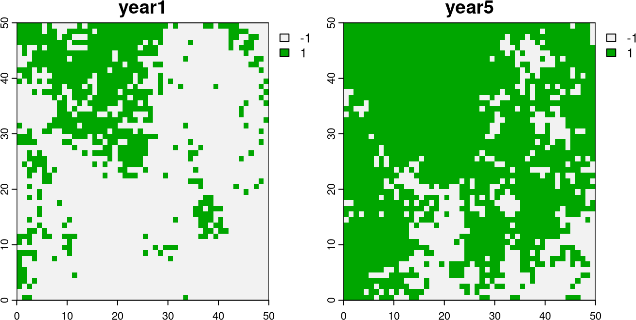
plot(c(map1, map2))
Optimizing the parameters
In this case, we have two maps: the first map (map1) is the initial map, and the second map (map2) is the expected map. Our main goal is to find the best values of B and J that, given the initial map (map1), will result in a simulated map that is as similar as possible to the expected map (map2).
One possible approach to find these best values of B and J is to use an optimization algorithm. This algorithm’s goal is to minimize the difference between the metrics of the expected map (e.g., map2) and the metrics of the last simulation.
For that purpose, we can use the optim_sa() function from the optimization package that implements the simulated annealing algorithm. Firstly, we need to define a function that takes one variable (x) and returns a single numeric value. Here, we created the optimize_model() function that takes the x variable, which is a vector of two values: B and J. The function then runs the spatial kinetic Ising model with the given values of B and J, calculates the composition and texture indexes for the expected map (map2) and the last simulation, and returns the distance between the metrics of the expected map (map2) and the metrics of the last simulation.1
optimize_model = function(x){
  sim = spatialising::kinetic_ising(x = map1, B = x[1], J = x[2],
                                    updates = 4)
  map2_metrics = c(composition_index(map2), texture_index(map2))
  sim_metrics = c(composition_index(sim[[4]]), texture_index(sim[[4]]))
  dist(rbind(map2_metrics, sim_metrics))[[1]]
}
Secondly, we need to use the optim_sa() function, which takes the optimize_model() function, the initial values of B and J, and the lower and upper bounds for B and J. Here, we set the bounds for B to be between 0 and 0.9 as we know that the proportion of the 1 (forest) values should increase over time. This operation may take about one minute in this case.
optim_params = optimization::optim_sa(fun = optimize_model,
                                      start = c(0.4, 0.4),
                                      lower = c(0, 0),
                                      upper = c(0.9, 0.9))
The output of the optim_sa() function is a list with several elements, including the best values of B and J in the par element.
optim_params$par[1] 0.78 0.51Here, our optimal values of B and J are 0.78 and 0.51, respectively. Now, we can use the newly derived values to simulate the spatial kinetic Ising model similar to the second map (map2).
sim_optim = kinetic_ising(map1,
                          B = optim_params$par[1], J = optim_params$par[2],
                          updates = 4)
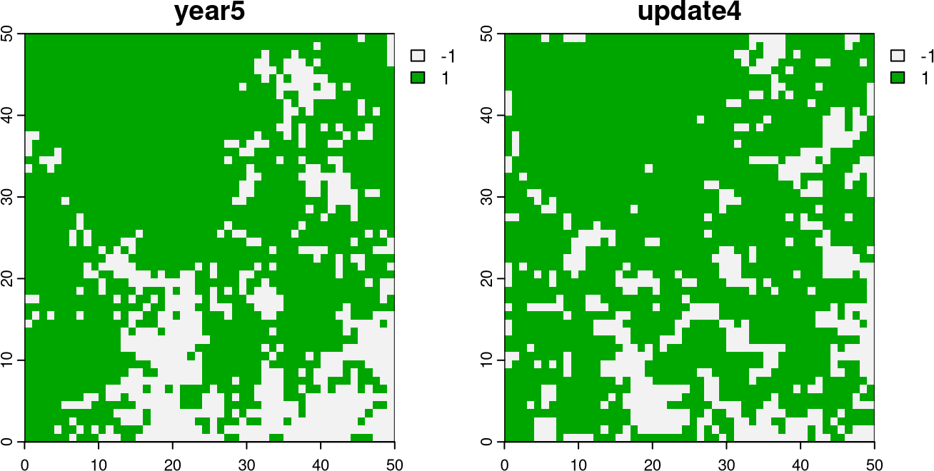
plot(c(map2, sim_optim[[4]]))
The map on the left is the expected, true map, and the map on the right is our simulation. While both maps are not identical, they have a similar spatial pattern with a dominance of forest (1) (especially in the northeast part of the map) and a similar configuration of the patches.
Exploring the simulation results
In addition to looking at just the final map, we can also retrace the entire simulation process and its effect on the metrics of spatial patterns. Firstly, we can plot all of the simulated rasters:
names(sim_optim) = paste0("sim_year", 2:5)
plot(sim_optim, nr = 1)
Secondly, we can calculate their metrics of spatial patterns and compare their changes over time.
ci_df = data.frame(year = 1:5, metric = "composition index",
                   value = composition_index(c(map1, sim_optim)))
ti_df = data.frame(year = 1:5, metric = "texture index",
                   value = texture_index(c(map1, sim_optim)))
pred_df = rbind(ci_df, ti_df)
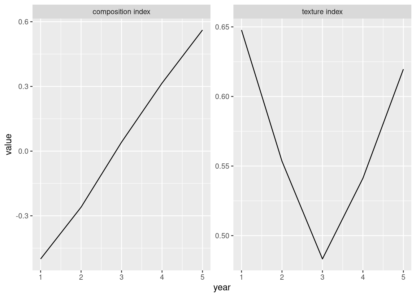
ggplot(pred_df, aes(year, value)) +
  geom_line() +
  facet_wrap(~metric, scales = "free_y")
As expected, the composition index increases over time, from negative values indicating a dominance of the -1 values to positive values indicating a dominance of the 1 values. The texture index, on the other hand, decreases for the first two simulations and then increases for the last two simulations. There is a good (and well-known) reason for that: the composition of values has an impact on the spatial texture. The larger the dominance of one category, the more clustered the values are, and thus the higher the texture index is.
Predicting the future changes
Given the assumption that the external pressure and the local autocorrelation tendency will remain the same, we can use the kinetic_ising() function to predict future spatial patterns.
map2_pred = kinetic_ising(map2,
                          B = optim_params$par[1], J = optim_params$par[2],
                          updates = 4)
names(map2_pred) = paste0("sim_year", 6:9)
plot(map2_pred, nr = 1)
The above map shows the predicted spatial patterns for the years 6, 7, 8, and 9.
Conclusions
This blog post showed how to use the simulated annealing algorithm to find the best values of B and J that minimize the difference between the metrics of the expected map and the metrics of the last simulation. It allows not only the simulation of spatial patterns similar to the expected map but also the analysis of the simulation process and prediction of future spatial patterns.
Of course, there are many caveats and limitations of this approach. For example, the spatial kinetic Ising model assumes that the external pressure and the local autocorrelation tendency are constant over time over the entire area. Moreover, the model is not able to simulate patterns that create or modify linear features (e.g., rivers or roads).
To learn more about the spatial kinetic Ising model, its background, possible applications, and limitations, I encourage you to read Stepinski (2023) and Stepinski and Nowosad (2023).
References
Footnotes
The optimization is also explained at https://jakubnowosad.com/spatialising/articles/Optimizing_spatialising_parameters.html.↩︎
Reuse
Citation
@online{nowosad2024,
  author = {Nowosad, Jakub},
  title = {Optimizing the Parameters of the Spatial Kinetic {Ising}
    Model to Simulate Spatial Patterns},
  date = {2024-01-07},
  url = {https://jakubnowosad.com/posts/2024-01-07-spatialising-bp2/},
  langid = {en}
}
