North Carolina SIDS data

(Use example(nc.sids) to read the data set from shapefile, together with import of two different list of neighbours). The nc.sids data frame has 100 rows and 21 columns. It contains data given in Cressie (1991, pp. 386-9), Cressie and Read (1985) and Cressie and Chan (1989) on sudden infant deaths in North Carolina for 1974-78 and 1979-84. The data set also contains the neighbour list given by Cressie and Chan (1989) omitting self-neighbours (ncCC89.nb), and the neighbour list given by Cressie and Read (1985) for contiguities (ncCR85.nb). The data are ordered by county ID number, not alphabetically as in the source tables sidspolys is a "polylist" object of polygon boundaries, and sidscents is a matrix of their centroids.

nc.sids

Format

This data frame contains the following columns:

• SP_ID: SpatialPolygons ID

• CNTY_ID: county ID

• east: eastings, county seat, miles, local projection

• north: northings, county seat, miles, local projection

• L_id: Cressie and Read (1985) L index

• M_id: Cressie and Read (1985) M index

• names: County names

• AREA: County polygon areas in degree units

• PERIMETER: County polygon perimeters in degree units

• CNTY_: Internal county ID

• NAME: County names

• FIPS: County ID

• FIPSNO: County ID

• CRESS_ID: Cressie papers ID

• BIR74: births, 1974-78

• SID74: SID deaths, 1974-78

• NWBIR74: non-white births, 1974-78

• BIR79: births, 1979-84

• SID79: SID deaths, 1979-84

• NWBIR79: non-white births, 1979-84

Source

Cressie, N (1991), Statistics for spatial data. New York: Wiley, pp. 386--389; Cressie, N, Chan NH (1989) Spatial modelling of regional variables. Journal of the American Statistical Association, 84, 393--401; Cressie, N, Read, TRC (1985) Do sudden infant deaths come in clusters? Statistics and Decisions Supplement Issue 2, 333--349; http://sal.agecon.uiuc.edu/datasets/sids.zip.

Examples

if (requireNamespace("sf", quietly = TRUE)) {
  if (requireNamespace("spdep", quietly = TRUE)) {
    library(spdep)
    nc.sids <- sf::st_read(system.file("shapes/sids.gpkg", package="spData")[1])
    row.names(nc.sids) <- as.character(nc.sids$FIPS)
    rn <- row.names(nc.sids)
    ncCC89_nb <- read.gal(system.file("weights/ncCC89.gal", package="spData")[1],
                          region.id=rn)
    ncCR85_nb <- read.gal(system.file("weights/ncCR85.gal", package="spData")[1],
                          region.id=rn)
                          
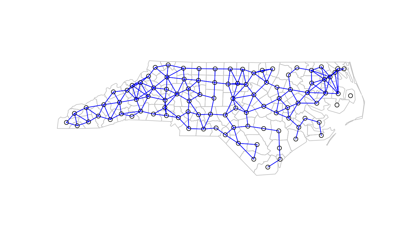
    plot(sf::st_geometry(nc.sids), border="grey")
    plot(ncCR85_nb, sf::st_geometry(nc.sids), add=TRUE, col="blue")
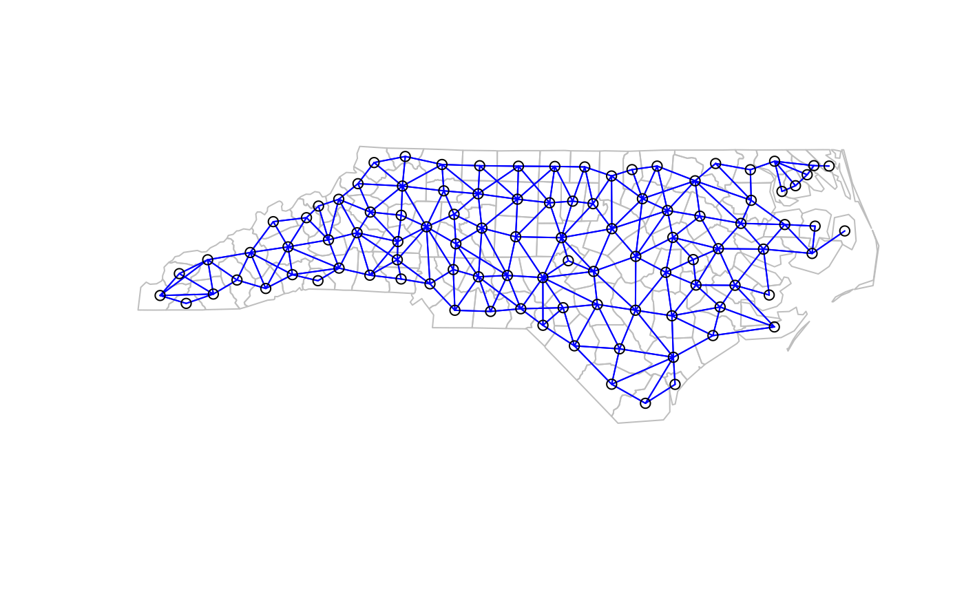
    plot(sf::st_geometry(nc.sids), border="grey")
    plot(ncCC89_nb, sf::st_geometry(nc.sids), add=TRUE, col="blue")
  }
}
#> Reading layer `sids' from data source 
#>   `/home/runner/work/_temp/Library/spData/shapes/sids.gpkg' using driver `GPKG'
#> Simple feature collection with 100 features and 22 fields
#> Geometry type: MULTIPOLYGON
#> Dimension:     XY
#> Bounding box:  xmin: -84.32385 ymin: 33.88199 xmax: -75.45698 ymax: 36.58965
#> Geodetic CRS:  NAD27
#> Warning: st_point_on_surface may not give correct results for longitude/latitude data

#> Warning: st_point_on_surface may not give correct results for longitude/latitude data