Spatial SHAP

The spatialexplain package provides model agnostic tools for exploring and explaining spatial machine learning models. This vignette shows a simple example of how to use it to explain a regression model with the Break Down method.

Lets start by attaching the necessary packages, reading the predictors raster, and loading the pre-trained regression model.

# attaching the necessary packages
library(spatialexplain)
library(terra)

# reading the predictors raster
predictors = rast("/vsicurl/https://github.com/Nowosad/IIIRqueR_workshop_materials/raw/refs/heads/main/data/predictors.tif")
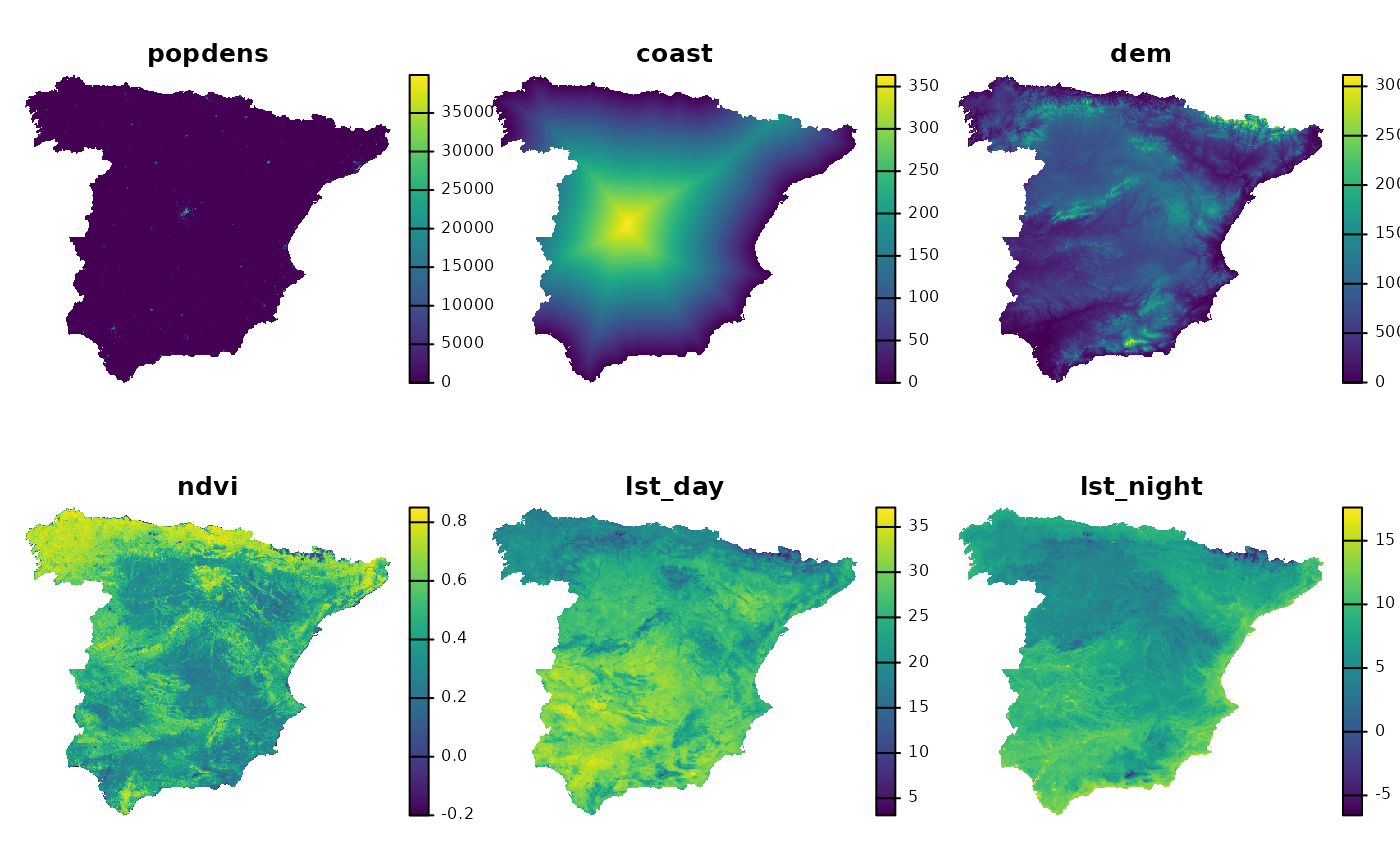
plot(predictors, axes = FALSE)


# loading the pre-trained regression model
data("regr_exp", package = "spatialexplain")
regr_exp
#> Model label:  rpart 
#> Model class:  rpart 
#> Data head  :
#>    popdens    coast      dem      ndvi  lst_day lst_night
#> 1 0.000000 1.126301 85.90540 0.3656146 24.37792  12.64256
#> 2 1.211701 6.743273 75.00126 0.3990190 28.13341  10.70668

The SHAP method is a model-agnostic method that explains the model’s predictions by attributing the prediction to each feature. However, as compared to the Break Down method, the SHAP method uses the idea of averaging the value of a variable’s attribution over all or many possible orderings. This has two main implications: the SHAP method is computationally more expensive, but its results are less sensitive to the order of the variables. This method provides additive feature attribution – thus, it works best for additive models (e.g., linear regression), and if the model is not additive, the SHAP values may not be meaningful.

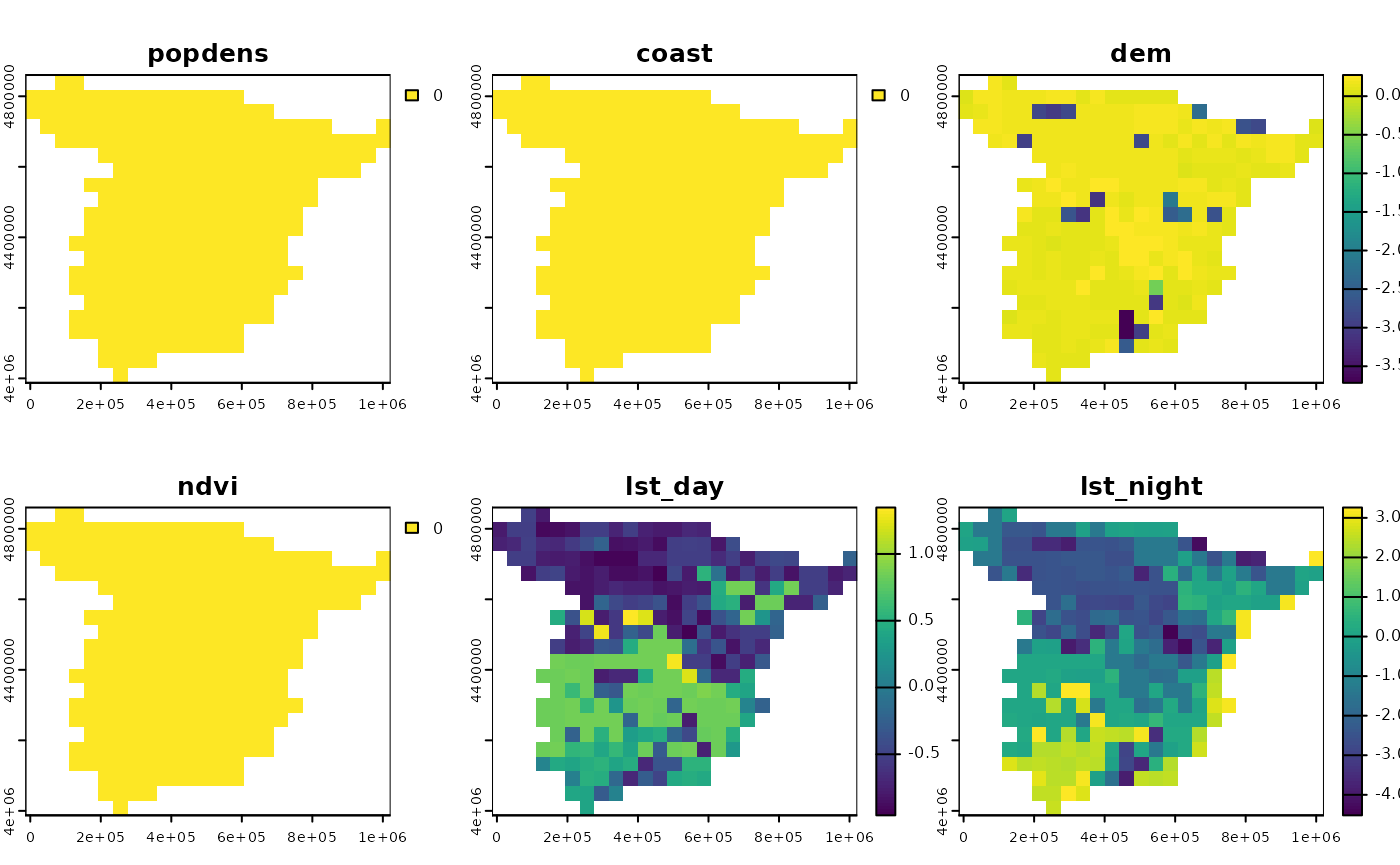
We can use the predict_spatial_parts() function to explain the regression model using the SHAP method by setting the type parameter to "shap".

regr_psp_shap = predict_spatial_parts(regr_exp, predictors, maxcell = 500,
                                      type = "shap")
plot(regr_psp_shap)

The resulting maps show that the popdens, coast, and ndvi variables had no effect on the model’s predictions. The dem variable mostly influenced the results in the mountainous areas, while lst_day and lst_night had different effects for the south and north parts of Spain.

For more explanation of the SHAP method, read the “Shapley Additive Explanations (SHAP) for Average Attributions” chapter from the Explanatory Model Analysis book.

Jakub Nowosad

2024-11-20