Geocomputation with R’s guide
to reproducible
spatial
data analysis

Jakub Nowosad, https://jakubnowosad.com/

OpenGeoHub Summer School 2022

2022-08-30

Chapter 1: Geocomputation

(geo)spati|graphic)*(al)*

( )*(stuff|data|comput|inform)*(ing|ation)*

(science|systems|theory|analysis)*

Based on the David O’Sullivan’s talk title at the Geocomputation 2019 conference

(geo)spati|graphic)*(al)*

( )*(stuff|data|comput|inform)*(ing|ation)*

(science|systems|theory|analysis)*

Based on the David O’Sullivan’s talk title at the Geocomputation 2019 conference

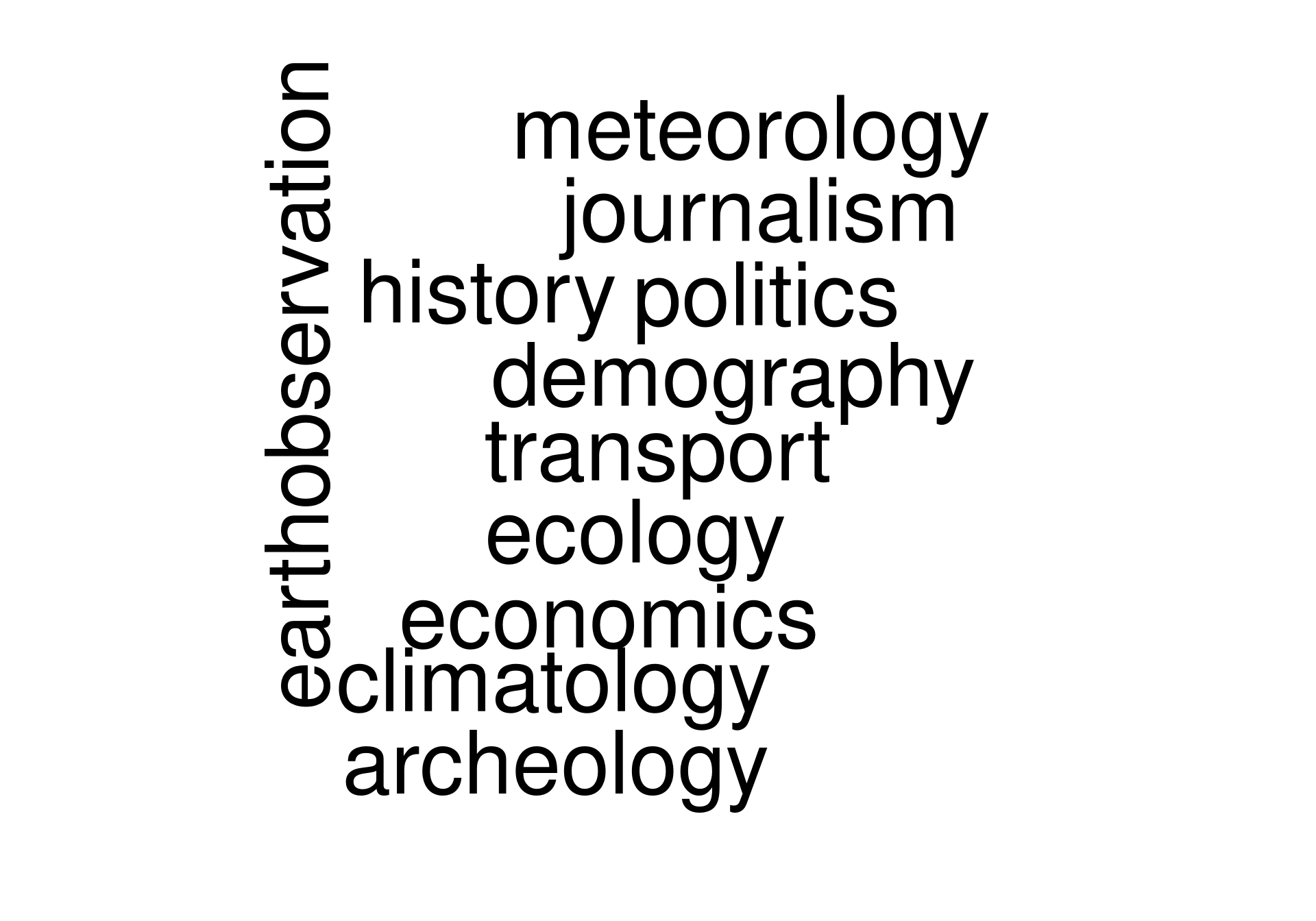
GeoComputation is about using the various different types of geodata and about developing relevant geo-tools within the overall context of a ‘scientific’ approach (Openshaw 2000).

At the turn of the 21st Century it was unrealistic to expect readers to be able to reproduce code examples, due to barriers preventing access to the necessary hardware, software and data

Differences in emphasis between software packages (Graphical User Interface (GUI) of Geographic Information Systems (GIS) and R).

Attribute	Desktop GIS (GUI)	R
Home disciplines	Geography	Computing, Statistics
Software focus	Graphical User Interface	Command line
Reproducibility	Minimal	Maximal

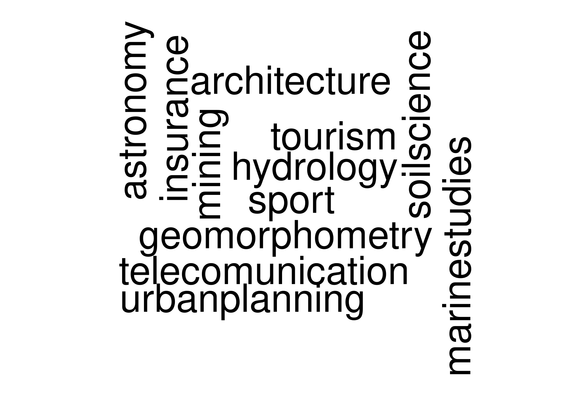
GIS Applications

Data models

Traditionally, spatial data is described by two basic data models:

• vector data model aimed at representing the world using points, lines, and polygons
• raster data model focused on representing surfaces

Vector data model(s)

Source: https://r-tmap.github.io/

Raster data model(s)

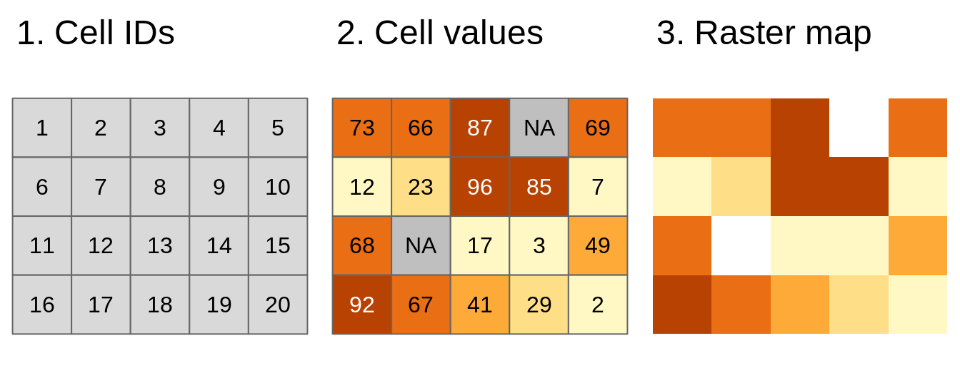
Source: https://r-tmap.github.io/

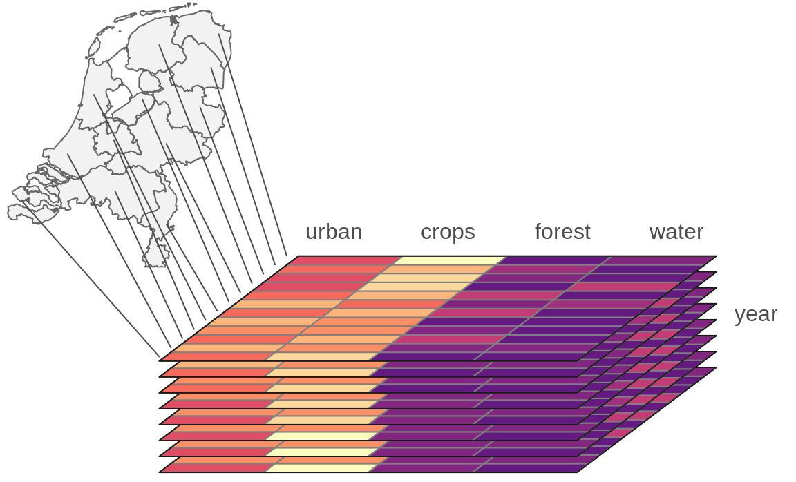
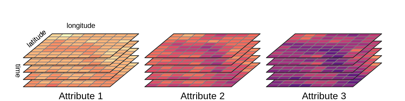
Spatial data cubes

Source: https://r-tmap.github.io/

Source: https://r-tmap.github.io/

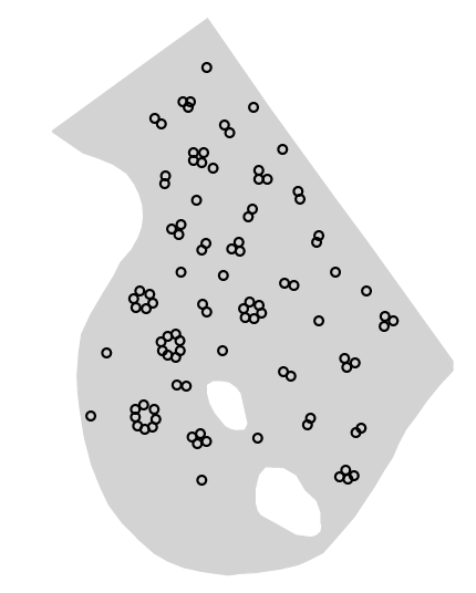
Point clouds

Source: https://github.com/Jean-Romain/lidR

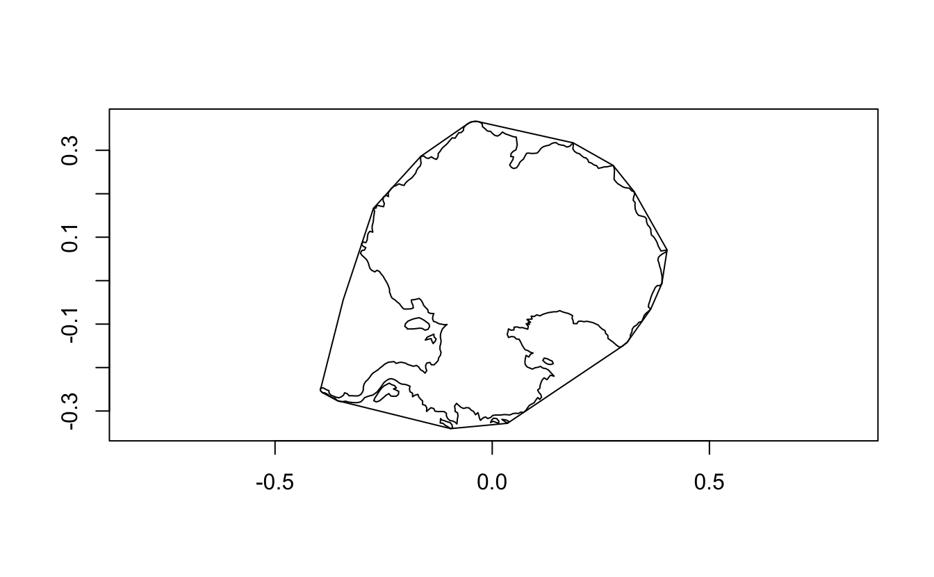
Coordinate reference systems

Geographic coordinates

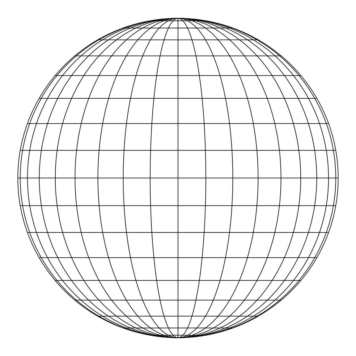
Projected coordinates

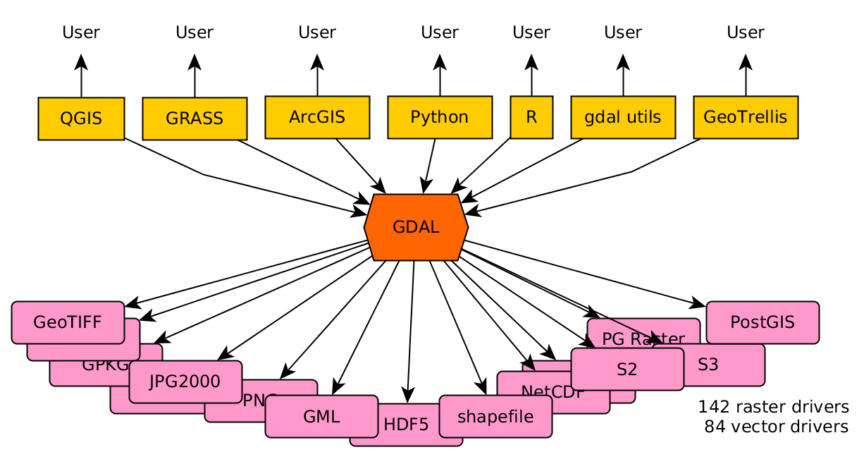
Data sources

Software databases:

File formats:

Source: https://r-spatial.org/2016/11/29/openeo.html

Data sources

Name	Extension	Model
ESRI Shapefile	.shp (the main file)	Partially open
GeoJSON	.geojson	Open
KML	.kml	Open
GPX	.gpx	Open
FlatGeobuf	.fgb	Open

Selected spatial file formats

Name	Extension	Model
GeoTIFF	.tif/.tiff	Open
Arc ASCII	.asc	Open
SQLite/SpatiaLite	.sqlite	Open
ESRI FileGDB	.gdb	Proprietary
GeoPackage	.gpkg	Open

Data sources

GDAL:

Source: https://r-spatial.org/2016/11/29/openeo.html

Data sources – new developments

SpatioTemporal Asset Catalog (STAC) – a general description format for spatiotemporal data that is used to describe a variety of datasets on cloud platforms including imagery, synthetic aperture radar (SAR) data, and point clouds.

Cloud Optimized GeoTIFF (COG) – raster objects saved as COGs can be hosted on HTTP servers, so other people can read only parts of the file without downloading the whole file

Other new file formats – GeoParquet, GeoArrow, Zarr

https://geocompr.robinlovelace.net/gis.html#stac-cogs-and-data-cubes-in-the-cloud, https://dewey.dunnington.ca/post/2022/building-bridges-arrow-parquet-and-geospatial-computing/

Data processing – basic vector operations

• Simplification
• Intersect
• Additional topological relations
• Spatial joins
• Centroids
• Buffers

Data processing – map algebra

Used for a various task related to spatial raster data.

It can be divided into four groups:

1. Local - per-cell operations
2. Focal (neighborhood operations) - most often the output cell value is the result of a 3 x 3 input cell block
3. Zonal operations - to summarize raster values for some zones (usually irregular areas)
4. Global - to summarize raster values for one or several rasters

Data processing – raster-vector interactions

1. Raster cropping and masking
2. Raster extraction - by points, lines, and polygons
3. Rasterization - points, lines, polygons to rasters
4. Vectorization - rasters to polygons or contours

Spatial data analysis

Based on the input data type:

Based on the goal of the analysis:

(incomplete lists)

Geocomputational methods

• Exploratory data analysis (EDA)
• Data processing (e.g., adding new variables)
• Data transformation (e.g., changing CRS, reducing size via simplification/aggregation)
• Data visualization
• Web application development
• Software development (e.g., to share new methods)

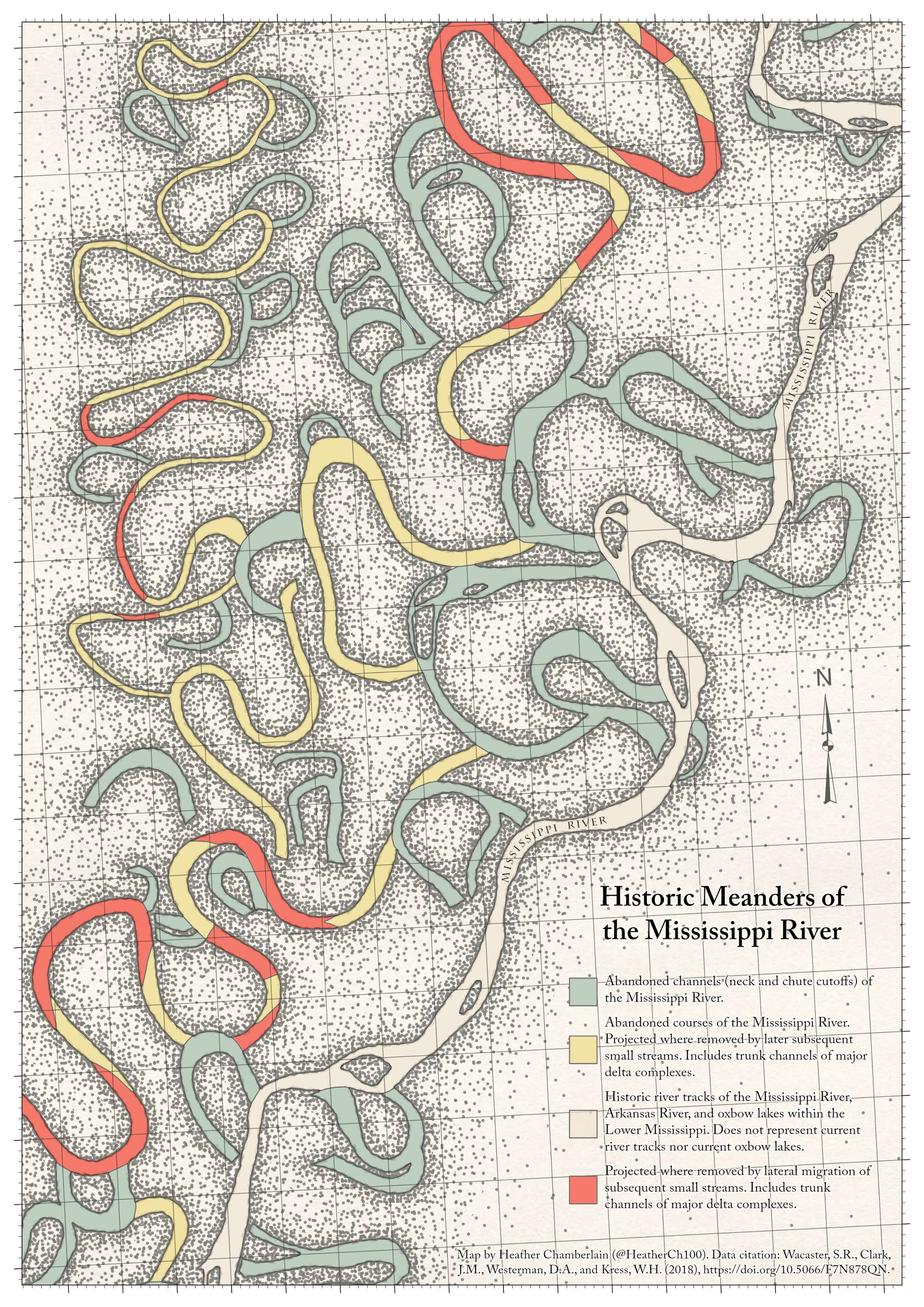
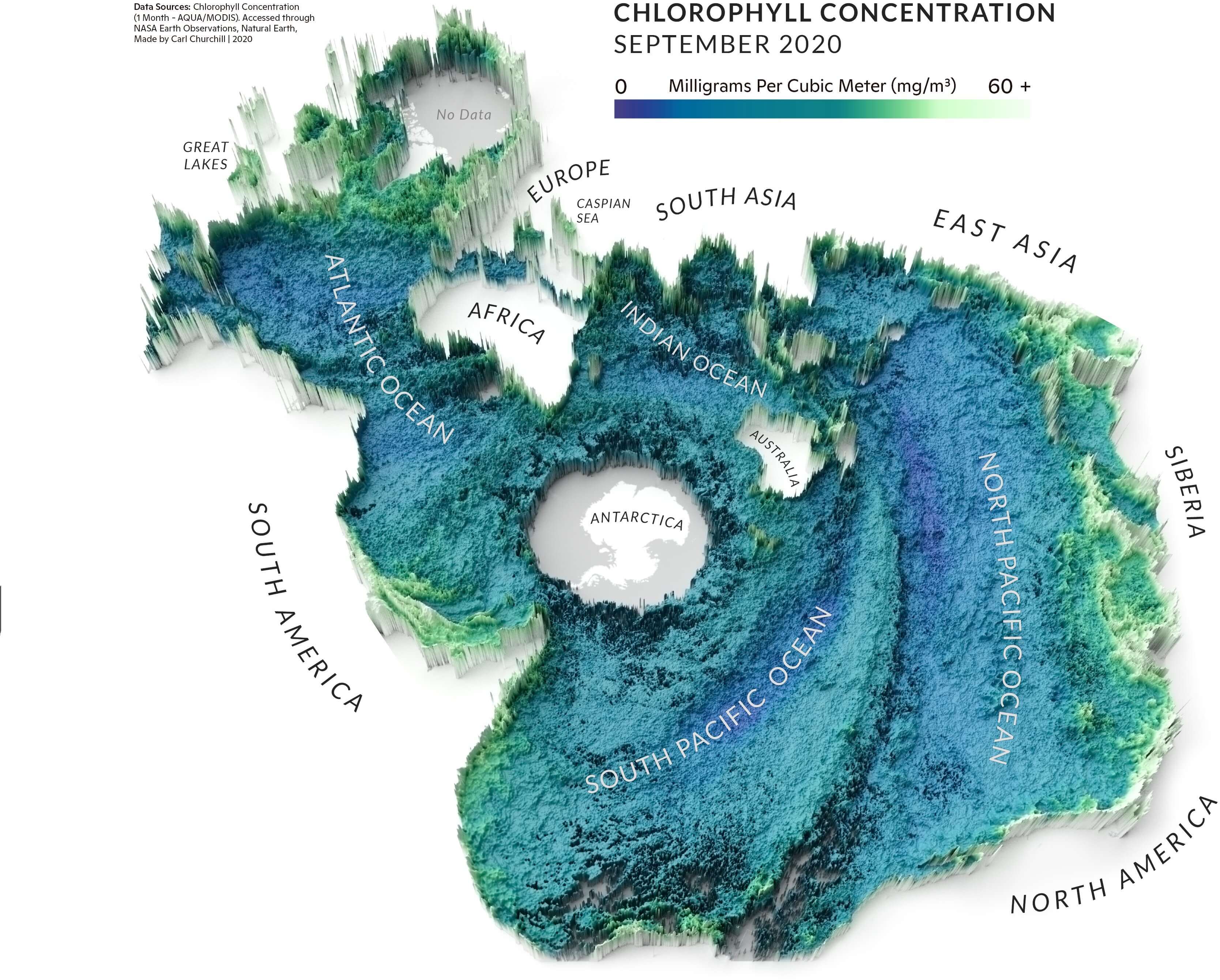
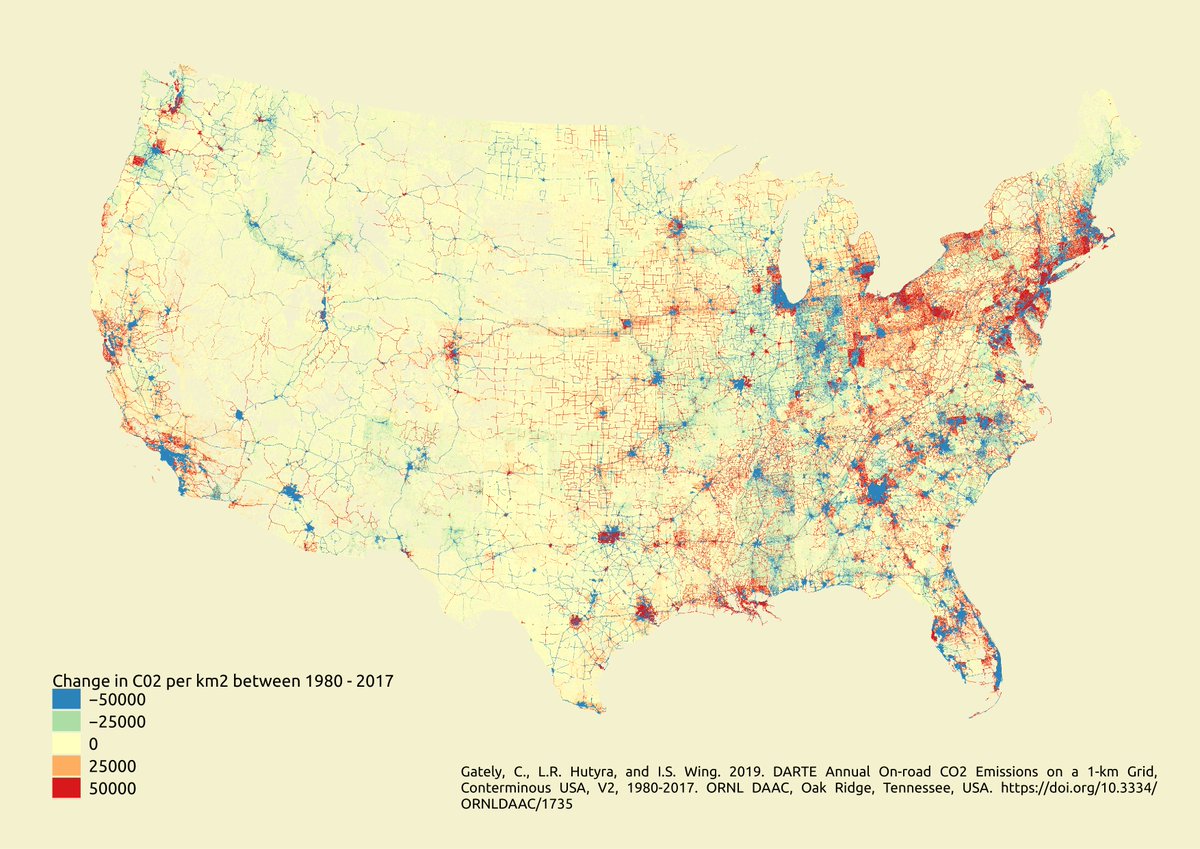
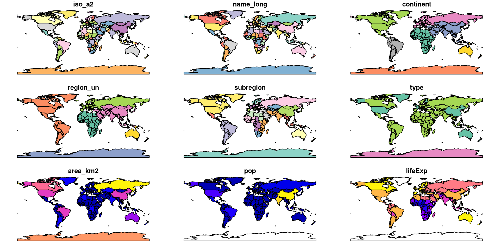
Spatial vizualizations

 

https://30daymapchallenge.com/2021/
@HeatherCh100, @Cchurchili, @@tjukanov, @evelynuuemaa

Chapter 2: Geocomputation with R

Ecosystems

“What a lawn” (CC BY-SA 2.0) by heipei …

“A field of flowers” (CC BY-SA 2.0) by Nigel Corby …

• {sf}, {sp}, {terra}, {raster}, {stars} - spatial classes
• {dplyr}, {rmapshaper} - processing of attribute tables/geometries
• {rnaturalearth}, {osmdata} - spatial data download
• {rgrass}, {qgisprocess}, {link2GI} - connecting with GIS software
• {gstat}, {mlr3}, {CAST} - spatial data modeling
• {rasterVis}, {tmap}, {ggplot2} - static visualizations
• {leaflet}, {mapview}, {mapdeck} - interactive visualizations
• {spatstat}, {spdep}, {spatialreg}, {dismo}, {landscapemetrics}, {RStoolbox}, {rayshader}, {gdalcubes}, {sfnetworks} - different types of spatial data analysis
• many more…

Visit https://cran.r-project.org/view=Spatial to get an overview of different spatial tasks that can be solved using R.

Source: https://geocompr.robinlovelace.net

library(spData)
library(sf)
world

Simple feature collection with 177 features and 10 fields
Geometry type: MULTIPOLYGON
Dimension:     XY
Bounding box:  xmin: -180 ymin: -89.9 xmax: 180 ymax: 83.64513
Geodetic CRS:  WGS 84
# A tibble: 177 × 11
   iso_a2 name_l…¹ conti…² regio…³ subre…⁴ type  area_…⁵     pop lifeExp gdpPe…⁶
 * <chr>  <chr>    <chr>   <chr>   <chr>   <chr>   <dbl>   <dbl>   <dbl>   <dbl>
 1 FJ     Fiji     Oceania Oceania Melane… Sove…  1.93e4  8.86e5    70.0   8222.
 2 TZ     Tanzania Africa  Africa  Easter… Sove…  9.33e5  5.22e7    64.2   2402.
 3 EH     Western… Africa  Africa  Northe… Inde…  9.63e4 NA         NA       NA 
 4 CA     Canada   North … Americ… Northe… Sove…  1.00e7  3.55e7    82.0  43079.
 5 US     United … North … Americ… Northe… Coun…  9.51e6  3.19e8    78.8  51922.
 6 KZ     Kazakhs… Asia    Asia    Centra… Sove…  2.73e6  1.73e7    71.6  23587.
 7 UZ     Uzbekis… Asia    Asia    Centra… Sove…  4.61e5  3.08e7    71.0   5371.
 8 PG     Papua N… Oceania Oceania Melane… Sove…  4.65e5  7.76e6    65.2   3709.
 9 ID     Indones… Asia    Asia    South-… Sove…  1.82e6  2.55e8    68.9  10003.
10 AR     Argenti… South … Americ… South … Sove…  2.78e6  4.30e7    76.3  18798.
# … with 167 more rows, 1 more variable: geom <MULTIPOLYGON [°]>, and
#   abbreviated variable names ¹​name_long, ²​continent, ³​region_un, ⁴​subregion,
#   ⁵​area_km2, ⁶​gdpPercap
# ℹ Use `print(n = ...)` to see more rows, and `colnames()` to see all variable names

plot(world)

Source: https://www.r-spatial.org/r/2020/03/17/wkt.html

library(terra)
srtm = rast(system.file("raster/srtm.tif", package = "spDataLarge"))
srtm

class       : SpatRaster 
dimensions  : 457, 465, 1  (nrow, ncol, nlyr)
resolution  : 0.0008333333, 0.0008333333  (x, y)
extent      : -113.2396, -112.8521, 37.13208, 37.51292  (xmin, xmax, ymin, ymax)
coord. ref. : lon/lat WGS 84 (EPSG:4326) 
source      : srtm.tif 
name        : srtm 
min value   : 1024 
max value   : 2892 

plot(srtm)

rspatial vs r-spatial

Legacy

Old vs New

Various R ecosystems

Other foundations

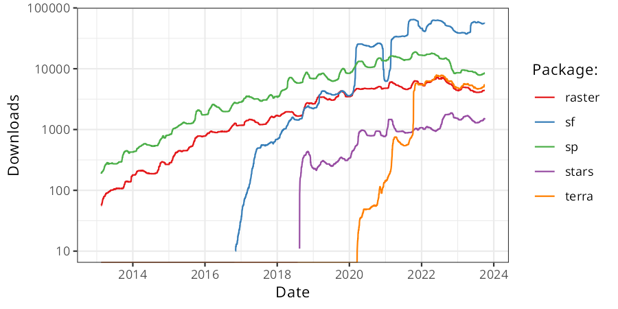
{stars} - https://r-spatial.github.io/stars/

{s2} - https://r-spatial.github.io/s2/

{lidR} - https://github.com/r-lidar/lidR

{sfnetwork} - https://luukvdmeer.github.io/sfnetworks

{spatstat} - https://spatstat.org/

hypertidy-verse - https://github.com/hypertidy

(Dependent) spatial packages

{supercells}

library(supercells)
library(terra)
s = rast(system.file("ex/logo.tif", package = "terra"))   
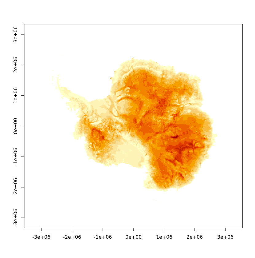
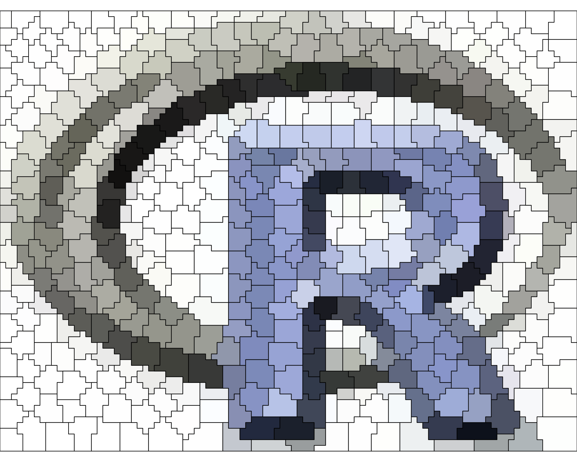
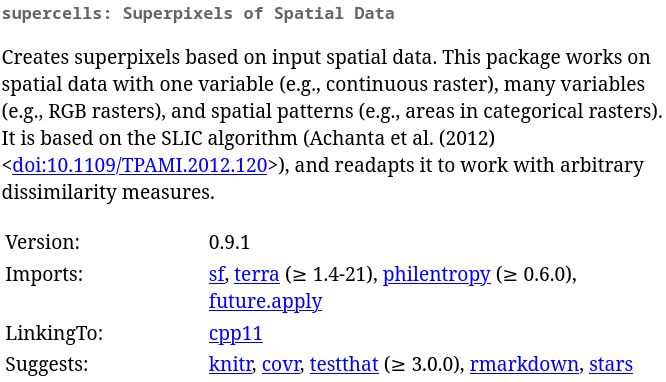
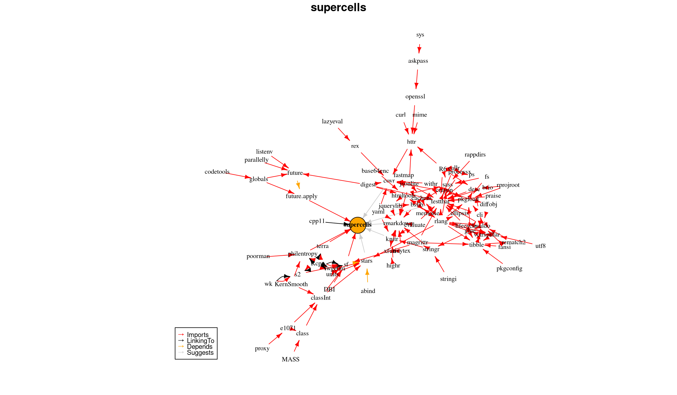
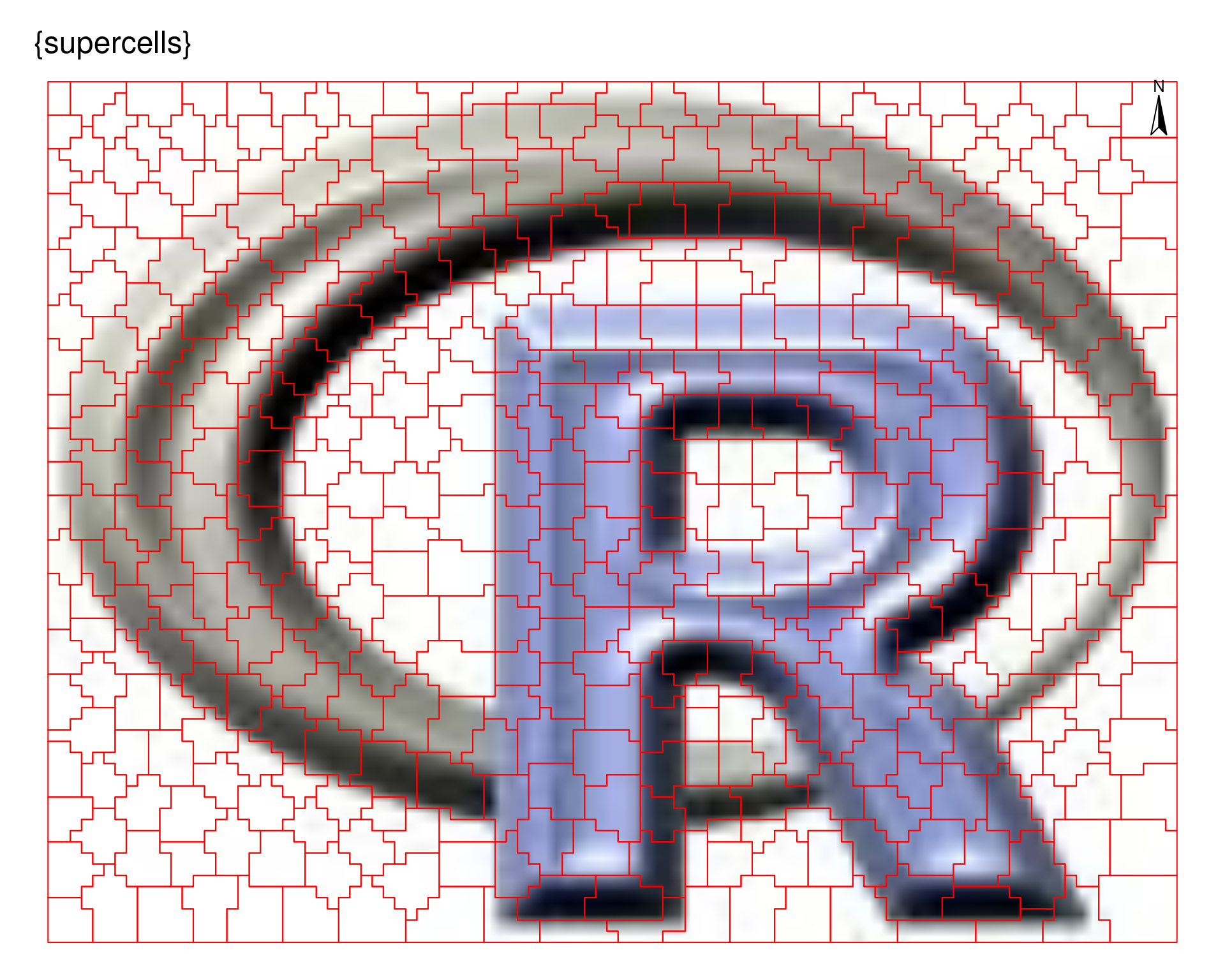
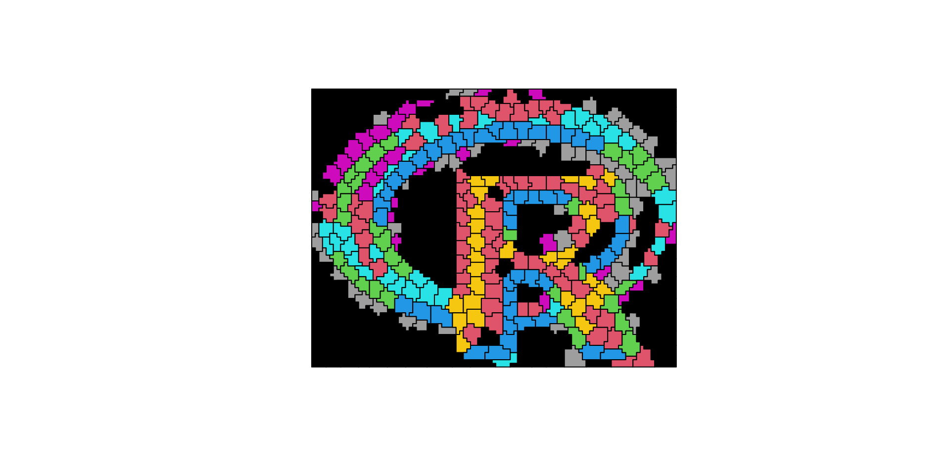
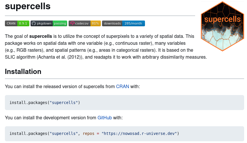
sc = supercells(s, 500, compactness = 50, transform = "to_LAB")

“Spidery Fence” (CC BY-NC-SA 2.0) by Theen …

“world’s largest spider web” (CC BY-NC-SA 2.0) by bluehurricane

Spatial vizualizations

https://r-tmap.github.io/

library(tmap)
tm_shape(s) +
  tm_rgb() +
  tm_shape(sc) +
  tm_borders(col = "red") +
  tm_compass(position = c("right", "top")) +
  tm_layout(main.title = "{supercells}",
            frame = FALSE)

Also see: tmap_mode("view"), {mapview}

Exercises

Easy

Medium

Hard

Chapter 3: Reproducible analysis

Reproduciblity spectrum

Based on: https://doi.org/10.1126/science.1213847

• Reproducible/Replicable
• Not only for publications!

Yes, but why?

Internal and external reasons

Self-reproduciblity

• To reproduce
• To replicate
• To fix/update/modify

• To extend
• To share
• (To not repeat ourselves)

External reproduciblity

• Reproducible
• Robust
• Transparent
• Reusable
• Shareable

Source: “Putting the R into Reproducible Research” by Anna Krystalli

Chapter 4: Reproducible geocomputation

Story of my life

• Issue: human memory
• http://dx.doi.org/10.2478/quageo-2014-0005
• Solution: code!

R code

library(terra)
library(supercells)
# setwd("")
s <- rast(system.file("ex/logo.tif", package = "terra"))   
sc = supercells(s, 500, compactness = 50,transform='to_LAB')
sck = kmeans(sf::st_drop_geometry(sc[4:6]), centers = 10)
plot(sf::st_geometry(sc[0]), col = sck$cluster)

• Issue: working directory
• Issue: code style
• Issue: randomness
• Issue: temporary objects

R code

RStudio: File > New Project > New Directory -> New Project -> …

Absolute vs relative paths

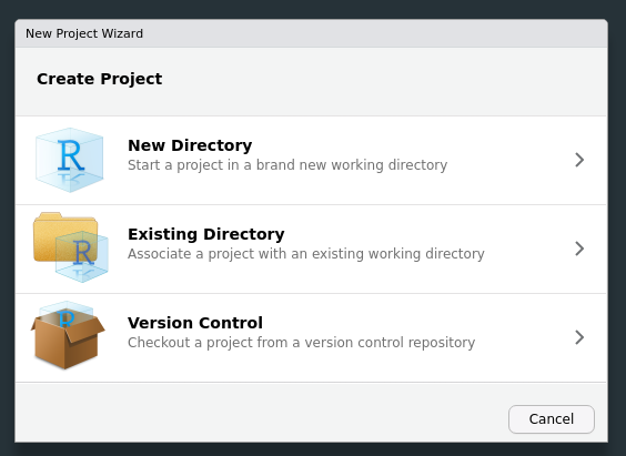
Also: clear environment + restart R

{reprex}: reproducible example

• Why: to ask a question; to report a bug; to fix a bug; to showcase some examples; …

• Input: minimal code allowing to reproduce your problem/example (strip away everything that is not directly related to your problem)

• Output: resulting runnable code + output as Markdown (including code results and plots) + (optionally) session info

https://twitter.com/robinlovelace/status/1561702311432523778

{reprex}: reproducible example

https://reprex.tidyverse.org/, https://community.rstudio.com/t/faq-whats-a-reproducible-example-reprex-and-how-do-i-create-one/5219

R code

• Issue: packages (and their dependencies) versions

{renv}

https://rstudio.github.io/renv/

1. renv::init() to initialize a new project-local environment with a private R library
2. Work in the project as normal, installing and removing new R packages
3. renv::snapshot() to save the state of the project library to the lockfile (renv.lock)
4. Continue working on your project
5. Call renv::snapshot() again to save the state of your project or renv::restore() to revert to the previous state as encoded in the lockfile

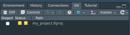
Version control

• Issue: what if the older version was better?
• Issue: backup copy
• Issue: sharing
• Issue: collaborating

Version control

Version control

https://github.com/Robinlovelace/geocompr

https://happygitwithr.com/

Literate programming

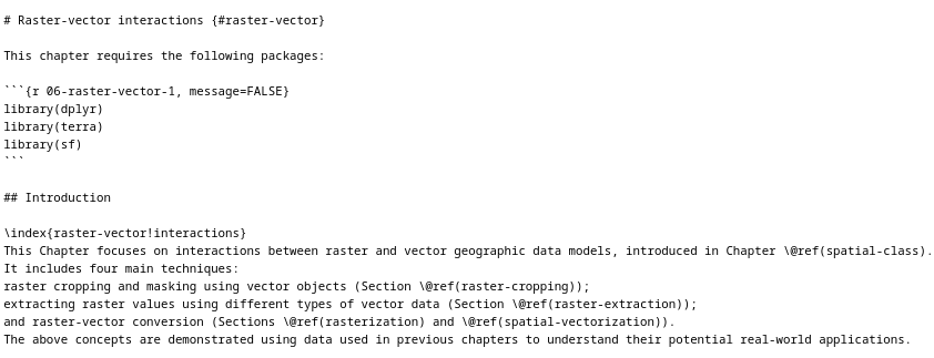
https://github.com/Robinlovelace/geocompr/blob/main/06-raster-vector.Rmd

Literate programming

https://geocompr.robinlovelace.net/raster-vector.html

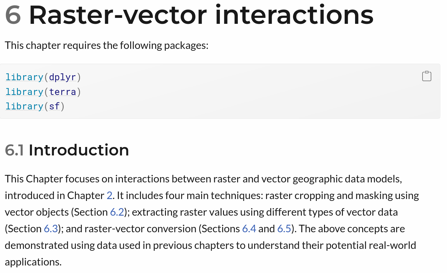
Literate programming

Writing Technical Papers with Markdown by Dheepak Krishnamurthy

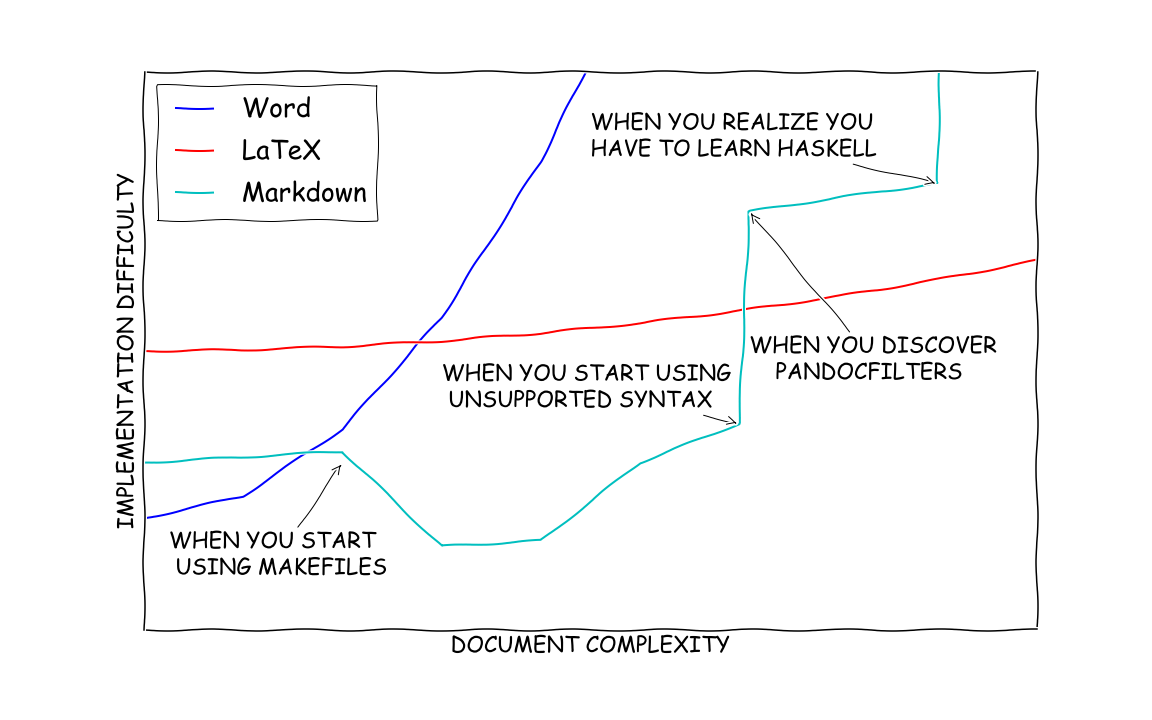
• Issue: create (and update) scientific and technical documents
• Markdown keeps everything (including text, code, figures, etc.) in one place
• Markdown supports reproducibility
• Markdown allows for more complexity (story of my life, again…)

https://rmarkdown.rstudio.com/, https://quarto.org/

{targets}

• Issue: large data
• Issue: computationaly demanding operations
• The {targets} package creates a reproducible workflow
• It skips costly runtime for tasks that are already up to date
• It allows to easy parallelization of the tasks

https://books.ropensci.org/targets/

{targets}

Before new changes: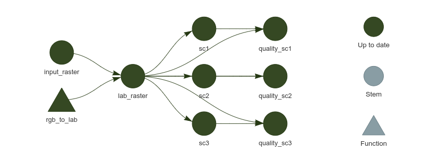

After new changes: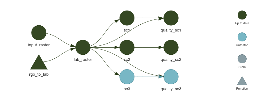

https://github.com/Nowosad/ogh2022-targets

R packages

• Issue: a lot of copy/paste or repeating ourselves
• Issue: no documentation

• Issue: problem with code sharing
• Issue: problem with example data sharing

R packages

R packages may serve many purposes…

https://github.com/Nowosad/supercells

https://github.com/Nowosad/spData https://github.com/geocompr/geocompkg

R packages

https://usethis.r-lib.org

Create a package template:

usethis::create_package("mypackage")

Subset of other useful {usethis} functions:

use_package("ggplot2", "Suggests")
use_readme_rmd()
use_mit_license("My Name")
use_data(x, y)
use_news_md()
use_test("my-test")

https://r-pkgs.org/, https://indrajeetpatil.github.io/awesome-r-pkgtools/

• Creating/modifying code (R/)
• Using the devtools::load_all() function, which loads new/modified functions into R session
• Verifying that the function works as expected using several examples (also adding unit tests)
• Updating the documentation of the code
• Generating documentation files using devtools::document()
• Checking if the package has any issues with devtools::check()
• Modifying the software version in the DESCRIPTION file
• Repeating the above steps

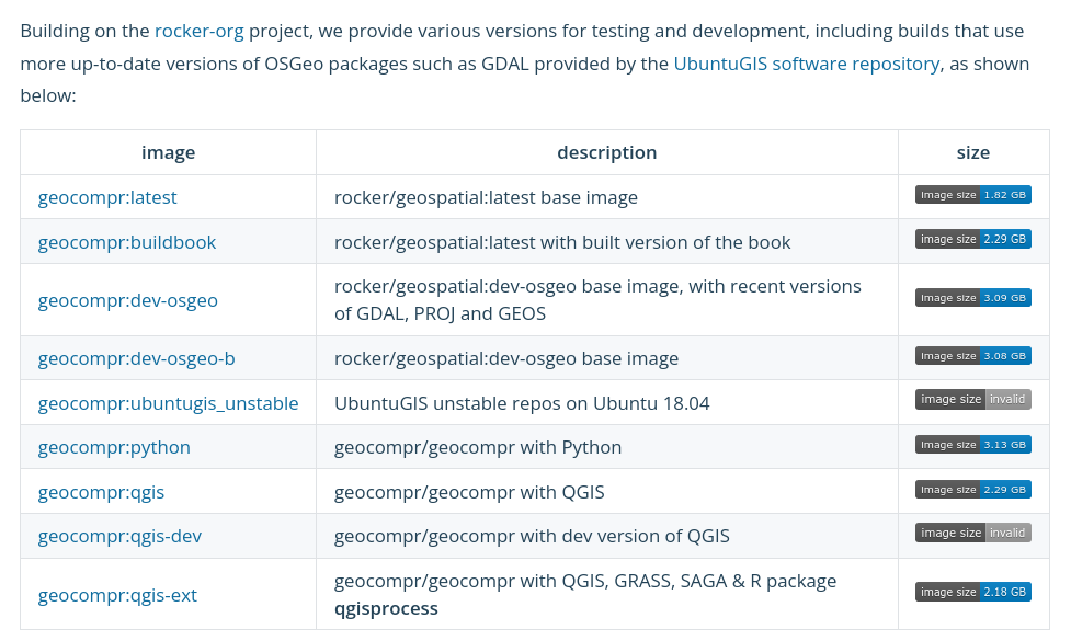
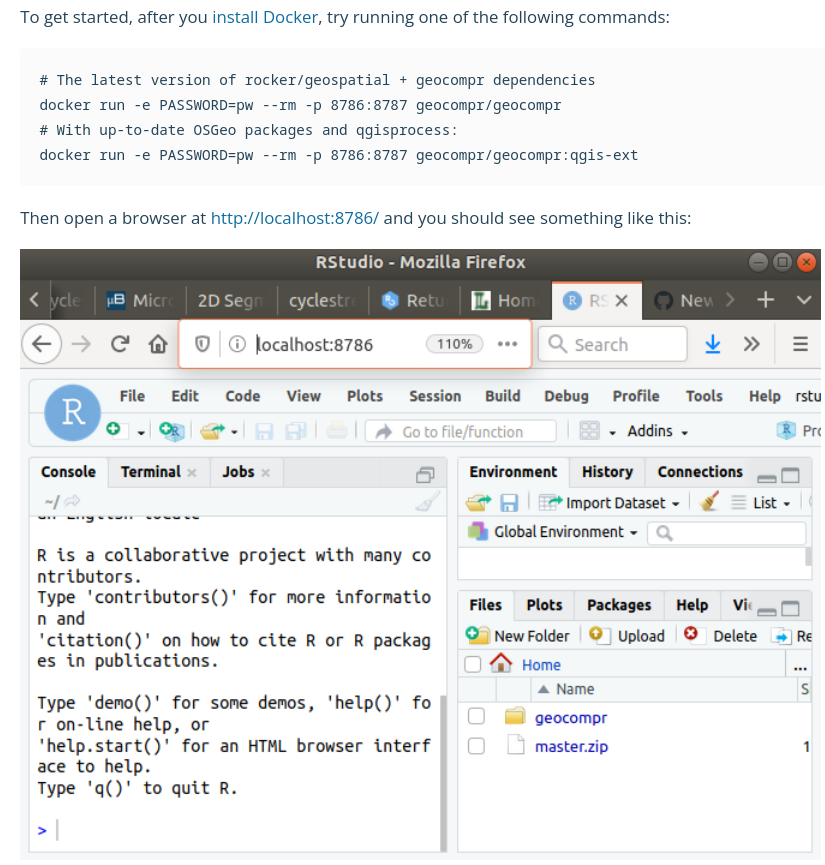
Docker

https://docs.docker.com/get-started/

https://hub.docker.com/r/geocompr/geocompr

Also see: https://mybinder.org/v2/gh/robinlovelace/geocompr/main?urlpath=rstudio

Also see: Create a Dockerfile from renv.lock – https://github.com/ThinkR-open/dockerfiler

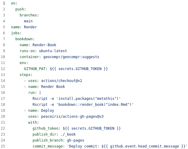
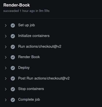
CI/CD

Issue: …but it works on my computer

CI/CD: continuous integration (CI) and continuous deployment (CD)

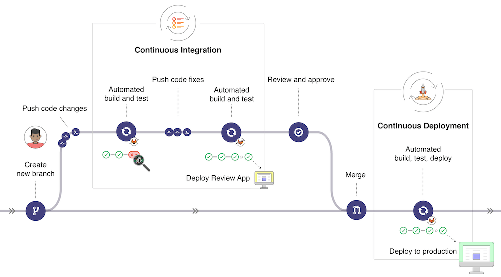
Source: https://docs.gitlab.com/ee/ci/introduction/

CI/CD

https://github.com/Robinlovelace/geocompr/blob/main/.github/workflows/main.yaml

https://geocompr.github.io/post/2022/geocompr-solutions/

Exercises

The end

https://jakubnowosad.com/ogh2022/