Spatial visualization with tmap

Jakub Nowosad (Adam Mickiewicz University, Poznań and University of Münster)

Earth Observation Summer School 2026, Istanbul, 2026-08-20

Setup

Slides and code: https://jakubnowosad.com/ogh2026/docs/tmap.html

install.packages(c("sf", "terra", "dplyr", "spData", "tmap", "tmap.mapgl"))

library(sf)
library(terra)
library(dplyr)
library(spData)
library(tmap)

R-spatial visualization ecosystem

R has a long history of supporting spatial data processing, analysis, and visualization

Spatial visualization packages include:

• rasterVis, mapsf, ggplot2 and ggspatial, tidyterra, rayshader – static visualizations
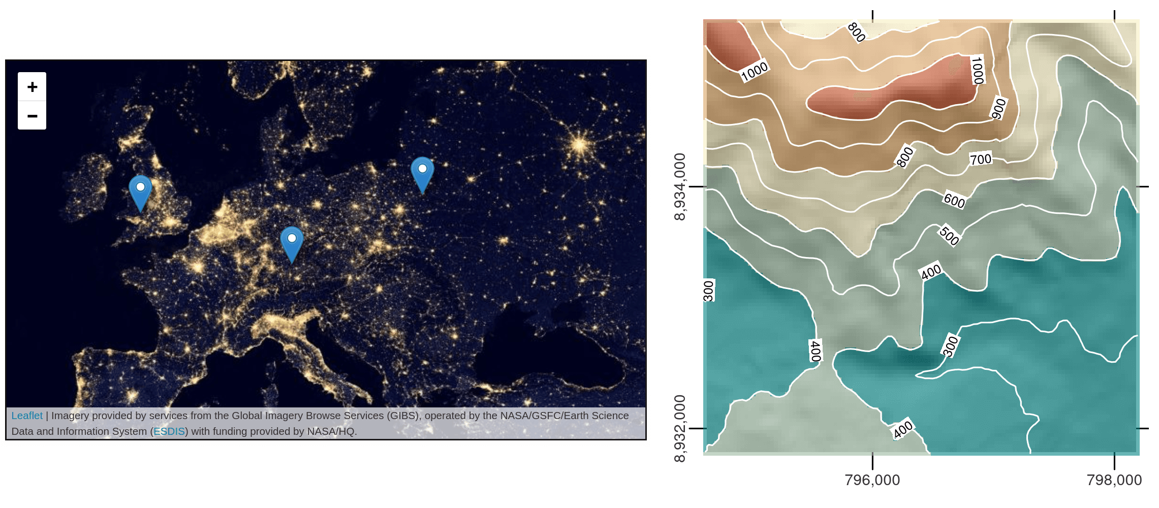
• leaflet, mapview, mapdeck, leafgl, mapgl – interactive visualizations
• tmap – both

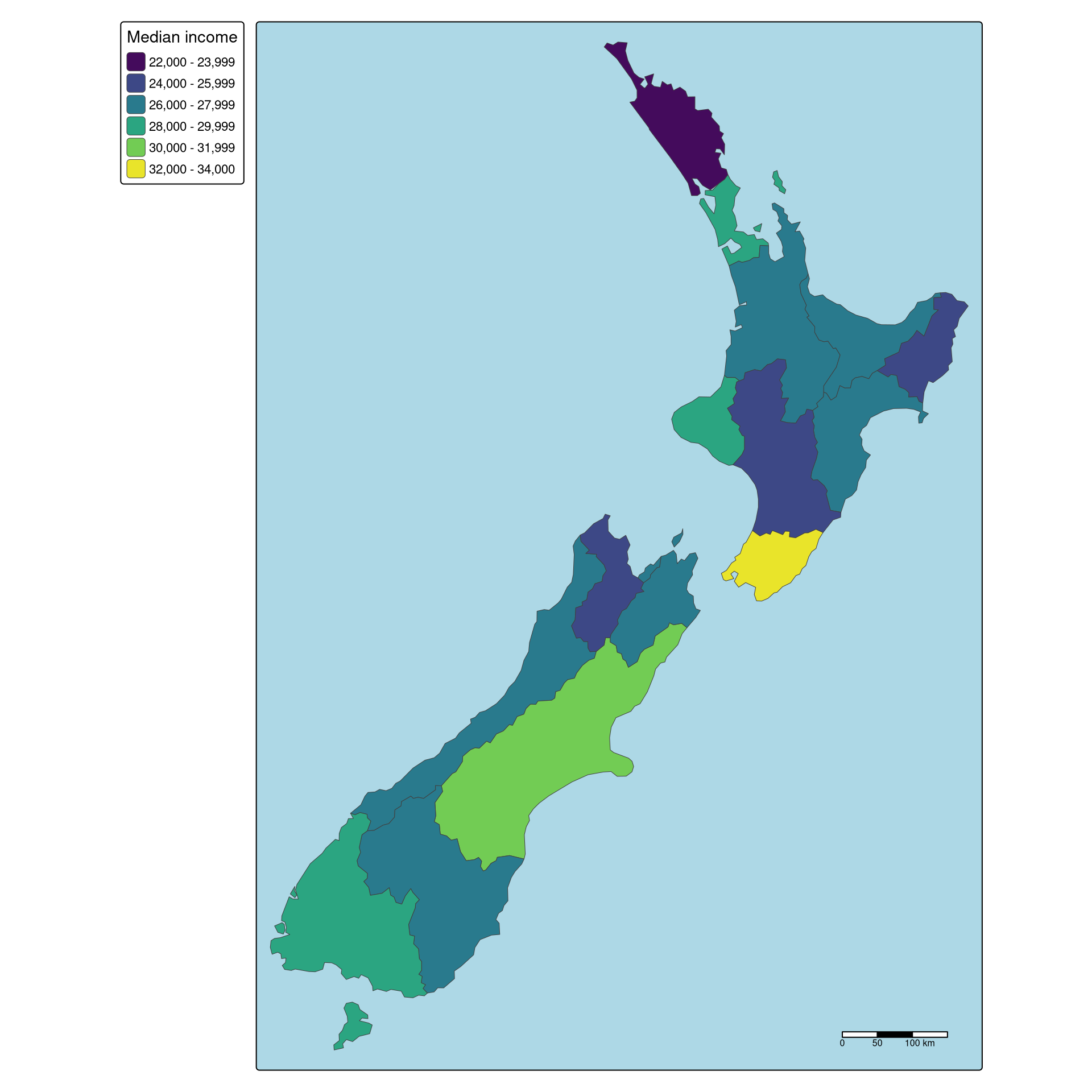
Anatomy of a {tmap} map

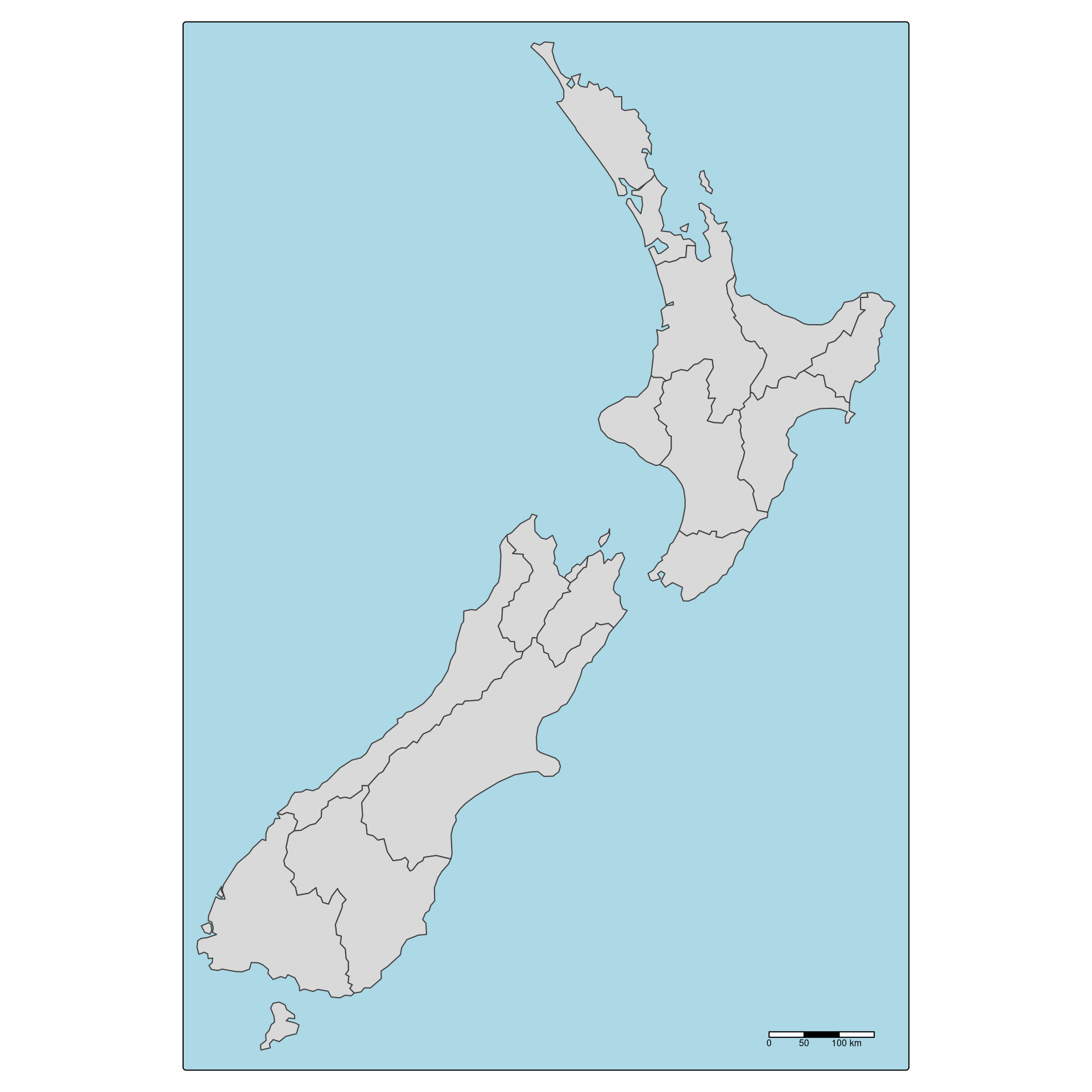
tm_shape(nz) +
  tm_polygons() +
  tm_scalebar() +
  tm_layout(bg.color = "lightblue")

Anatomy of a {tmap} map

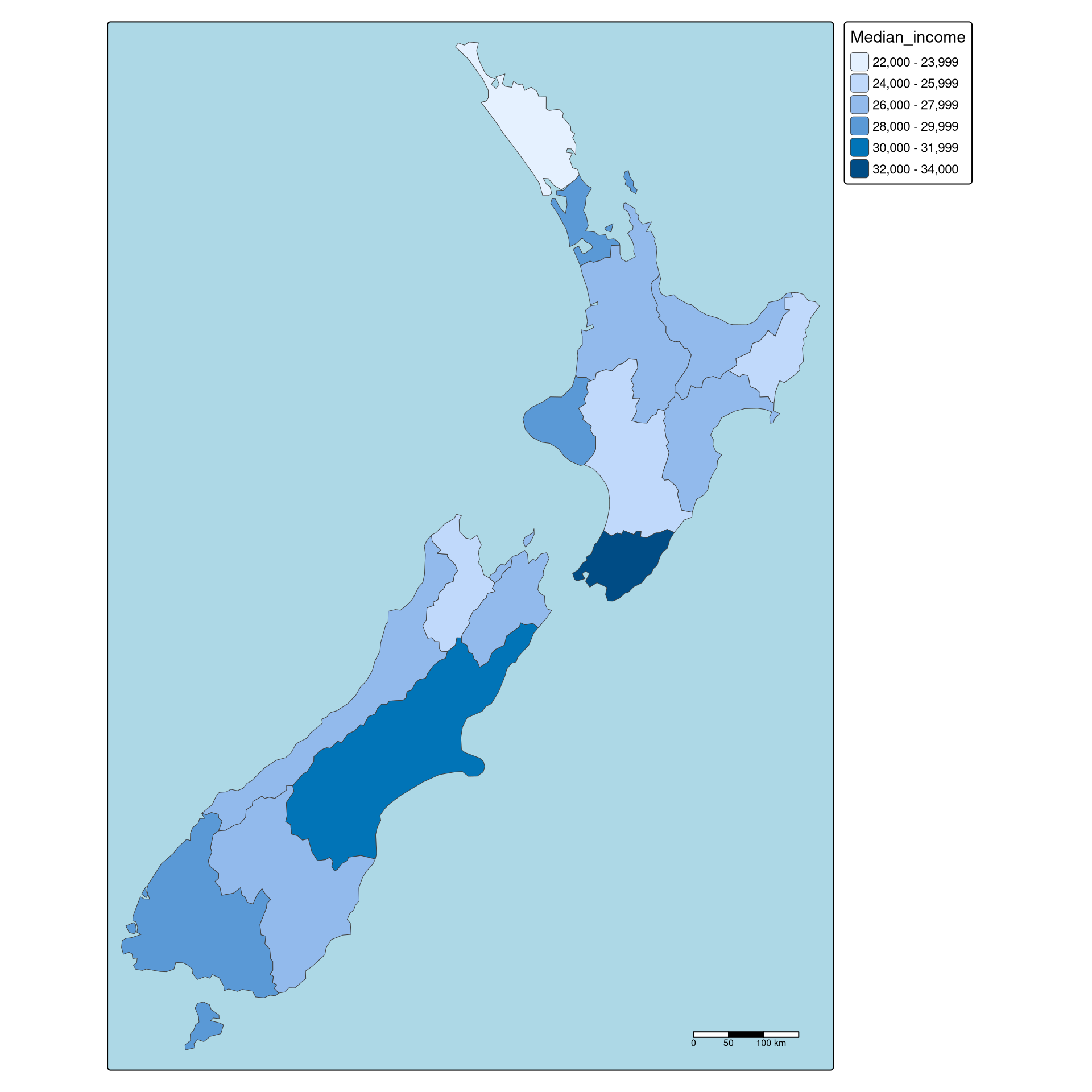
tm_shape(nz) +
  tm_polygons(
    fill = "Median_income",
    lwd = 0.5
  ) +
  tm_scalebar(
    position = c("right", "bottom")
  ) +
  tm_layout(bg.color = "lightblue")

Anatomy of a {tmap} map

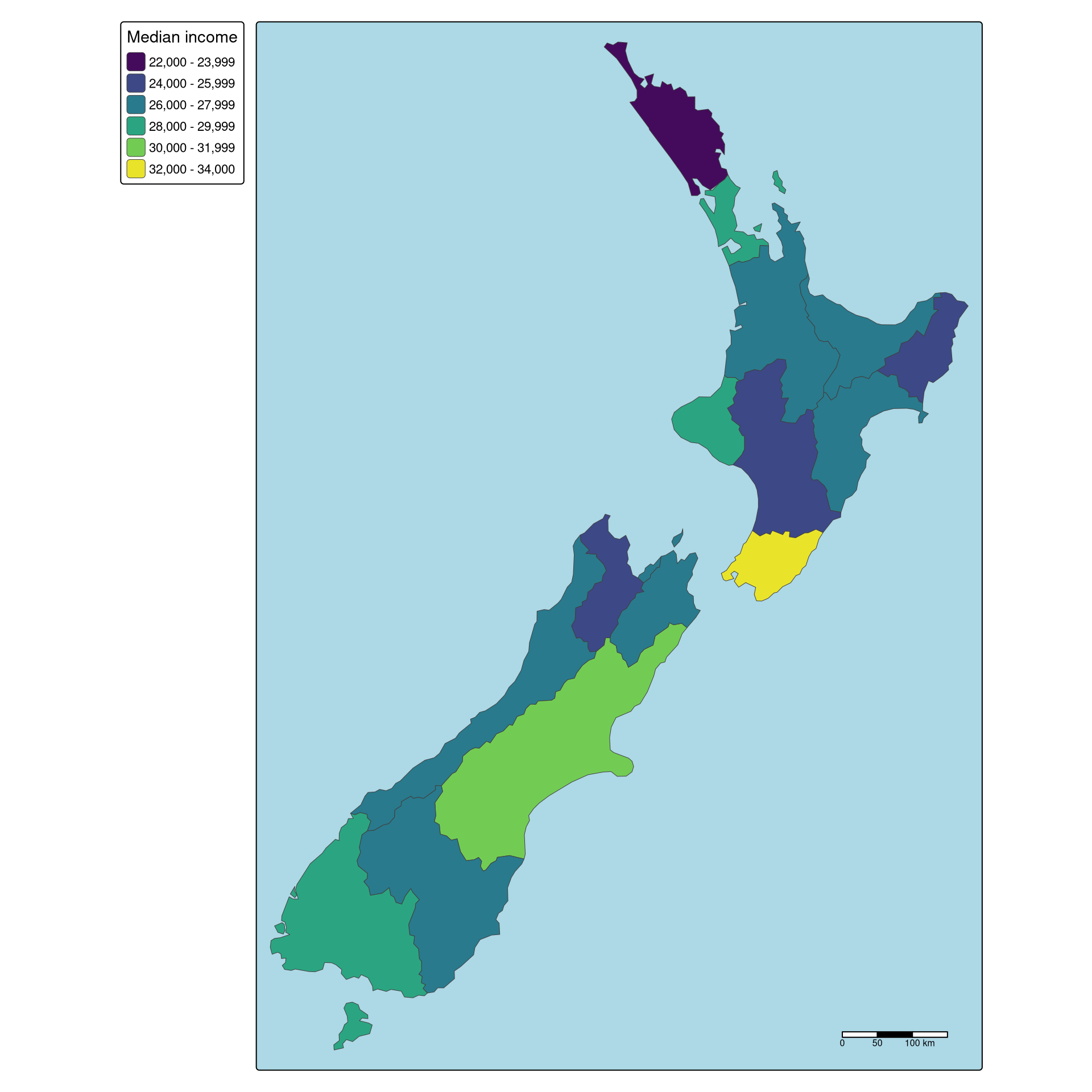
tm_shape(nz) +
  tm_polygons(
    fill = "Median_income",
    fill.scale = tm_scale(
      values = "viridis"
    ),
    fill.legend = tm_legend(
      title = "Median income",
      position = tm_pos_out(
        "left", "center"
      )
    ),
    lwd = 0.5
  ) +
  tm_scalebar(
    position = c("right", "bottom")
  ) +
  tm_layout(bg.color = "lightblue")

Anatomy of a {tmap} map

tm_shape(nz) +
  tm_polygons(
    fill = "Median_income",
    fill.scale = tm_scale(
      values = "viridis"
    ),
    fill.legend = tm_legend(
      title = "Median income",
      position = tm_pos_out(
        "left", "center"
      )
    ),
    lwd = 0.5
  ) +
  tm_scalebar(
    position = c("right", "bottom")
  ) +
  tm_layout(bg.color = "lightblue")

Anatomy of a {tmap} map

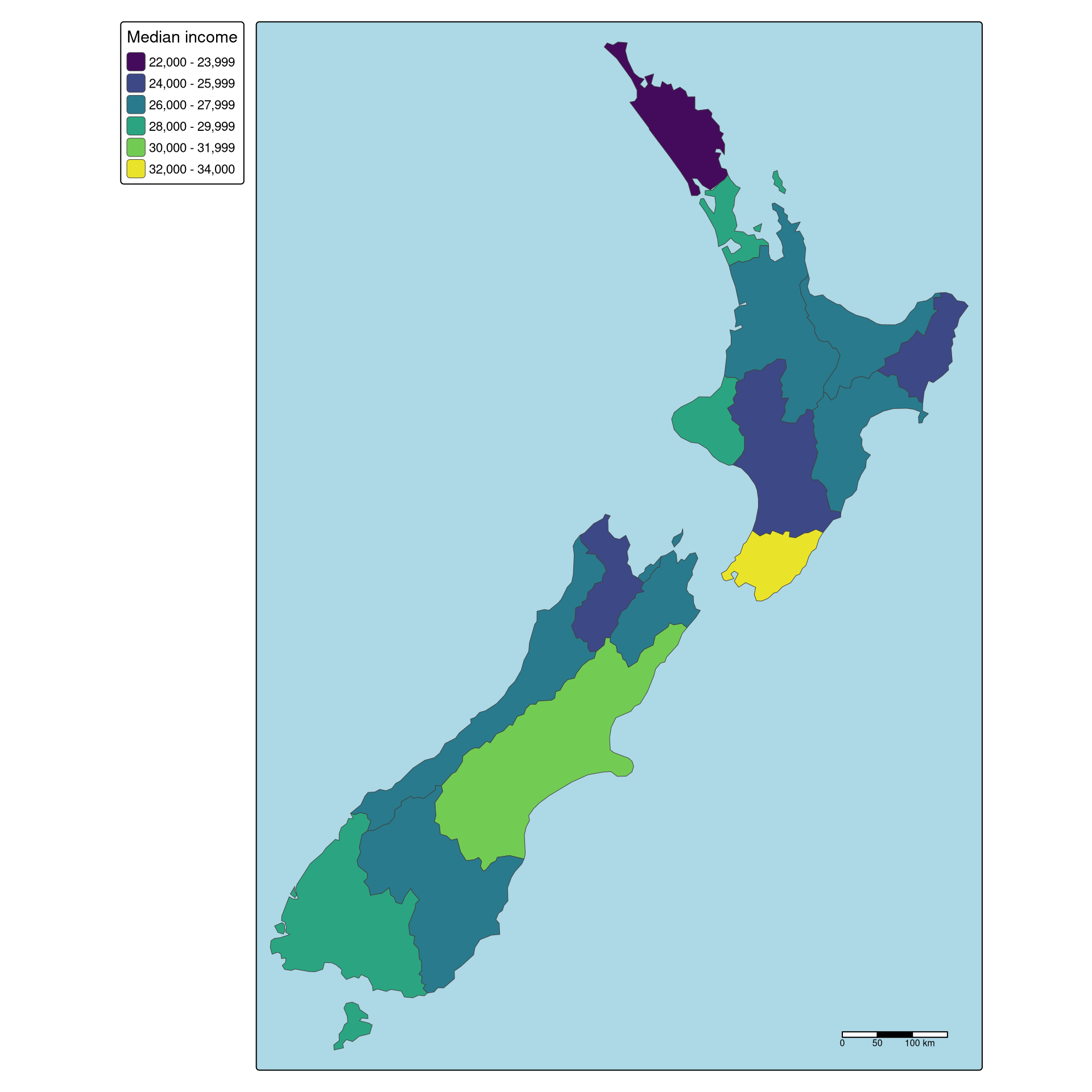
tm_shape(nz) +
  tm_polygons(
    fill = "Median_income",
    fill.scale = tm_scale(
      values = "viridis"
    ),
    fill.legend = tm_legend(
      title = "Median income",
      position = tm_pos_out(
        "left", "center"
      )
    ),
    lwd = 0.5
  ) +
  tm_scalebar(
    position = c("right", "bottom")
  ) +
  tm_layout(bg.color = "lightblue")

Main map layers

Function	Geometry	Map variables
tm_polygons()	polygons	fill, fill_alpha, col, col_alpha, lwd, lty
tm_symbols()	points, polygons, and lines	size, shape, fill, fill_alpha, col, col_alpha, lwd
tm_lines()	lines	col, col_alpha, lwd, lty
tm_text()	points, polygons, and lines	text, size, col, col_alpha, fontface
tm_raster()	raster	col, col_alpha

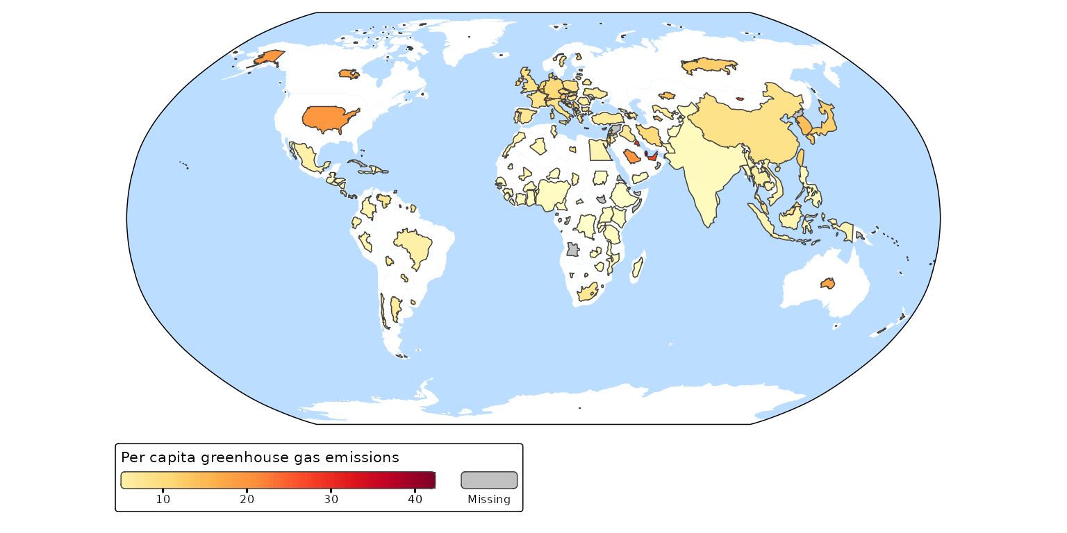
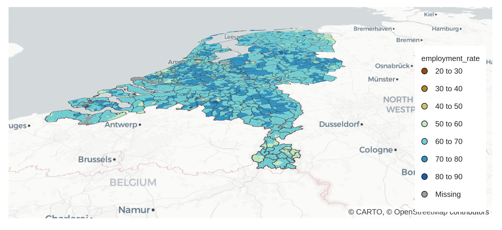
Each map layer can be constant or data-driven.

If data-driven, you may use .scale and .legend, for example, fill.scale and fill.legend in tm_polygons().

Main map components

Function	Description
tm_grid()	draws coordinate grid lines of the coordinate system of the main shape object
tm_graticules()	draws latitude and longitude graticules
tm_scalebar()	adds a scale bar
tm_compass()	adds a compass rose (north arrow)
tm_credits()	adds a text annotation
tm_logo()	adds a logo
tm_minimap()	adds minimap

Map components can be positioned inside or outside the map frame with:

• c("left", "center") for inside the map frame
• tm_pos_in() for inside the map frame
• tm_pos_out() for outside the map frame

Code examples

File: code/map_code1.R

File: code/map_code2.R

Exercises

Run the code below:

library(sf)
library(tmap)
library(spData)

The nz object contains a few attributes of regions within New Zealand.

1. Create a simple map of the nz data.
2. Improve the map by coloring regions based on their median income (Median_income). Improve the legend title. Try different color palettes (hint: use the fill.scale argument). Change border width. Put the legend on the left side.
3. Improve the map further by adding a title, scale bar, north arrow, and text annotation. Adjust the positions of map elements.
4. Switch to tmap_mode("view") and recreate the map from step 3. What are the pros and cons of static vs interactive maps?
5. Save the map as .png and .svg, and as .html.

Code examples (continued)

File: code/map_code3.R

File: code/map_code4.R

Advanced {tmap}

Website: https://r-tmap.github.io/tmap/

Book: https://tmap.geocompx.org/

Other features:

• Many other visual variables, e.g., tm_lines() and tm_raster()
• More complex scales for various data types
• Including charts (e.g., histograms) in the legend
• Adding inset maps
• Blending multiple layers
• Creating {shiny} apps with {tmap}
• Extensions of {tmap} to other layer types, data classes, or modes (e.g., tm_cartogram())

Summary

• {tmap} is a powerful R package for creating both static and interactive maps
• It follows a layered grammar of graphics: start with data, add layers, scales, legends, and update layout
• It excels at publication-quality static maps and quick interactive maps
• It is less suited to fully customized interactive dashboards, real-time streaming, or highly specialized cartographic design
• The R ecosystem offers many alternatives for spatial visualization
• Map making is iterative: consider your audience and purpose at every step
• Above all, making maps is a creative process

Contact

https://jakubnowosad.com

Resources

Website: https://r-tmap.github.io/tmap/

Book: https://tmap.geocompx.org/

Slides:

Acknowledgements