Calculation of growing degree days (GDD) in the pollen package

Growing degree days (GDD) are a measure of heat accumulation used to predict plant and animal development rates. It can be, however, calculated using several approaches. The pollen package allows for three different versions of the GDD calculations. The goal of this vignette is to describe and show examples of calculating GDD using different methods.

Let’s start with attaching a set of package used in this vignette:

library(pollen)
library(ggplot2)
library(tidyr)

Next, we will use the gdd_data dataset - a data frame with three columns:

day - this could be a date in real data
tmax - this value would represent a maximum temperature in real data
tmin - this value would represent a minimum temperature in real data

data("gdd_data", package = "pollen")
head(gdd_data)
#>   day tmax tmin
#> 1   1    2    2
#> 2   2    2    2
#> 3   3    2    2
#> 4   4    2    2
#> 5   5    2    2
#> 6   6    2    2

We can vizualize the gdd_data dataset using the ggplot2 package:

df_plot1 <- pivot_longer(gdd_data, tmax:tmin)
p1 <- ggplot(df_plot1) +
  geom_line(aes(day, value, color = name))
p1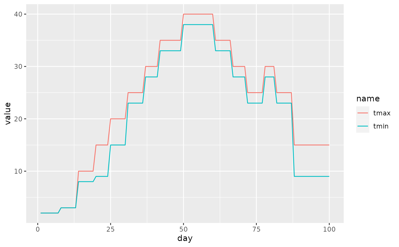

The pollen package allows for calculations of growing degree days (GDD) using the gdd() function. This function accepts up to five arguments:

tmax - daily maximum temperature
tmin - daily minimum temperature
tbase - base temperature
tbase_max - maximum base temperature
type - type of the GDD calculations. Either “B”, “C”, or “D”. The default is “C”.

The last argument is inspired by the article by Baskerville and Emin (1969) (see Figure 1 in the mentioned paper).

Type "B" - The heat units are calculated based on the difference between the mean daily temperature and the threshold (tbase). In the case when the value of tmin is lower than tbase, then it is replaced by tbase
Type "C" - same as type "B" and when the value of tmax is larger than tbase_max, then it is replaced by tbase_max
Type "D"- same as type "B" and when the value of tmax is larger than tbase_max, then no heat units are added

gdd_data$type_b <- gdd(tmax = gdd_data$tmax, tmin = gdd_data$tmin, 
                       tbase = 5, type = "B")
gdd_data$type_c <- gdd(tmax = gdd_data$tmax, tmin = gdd_data$tmin, 
                       tbase = 5, tbase_max = 20, type = "C")
gdd_data$type_d <- gdd(tmax = gdd_data$tmax, tmin = gdd_data$tmin, 
                       tbase = 5, tbase_max = 20, type = "D")
head(gdd_data)
#>   day tmax tmin type_b type_c type_d
#> 1   1    2    2      0      0      0
#> 2   2    2    2      0      0      0
#> 3   3    2    2      0      0      0
#> 4   4    2    2      0      0      0
#> 5   5    2    2      0      0      0
#> 6   6    2    2      0      0      0

Finally, let’s compare these three types:

df_plot2 <- pivot_longer(gdd_data, type_b:type_d)
p2 <- ggplot(df_plot2) +
  geom_line(aes(day, value, color = name))
p2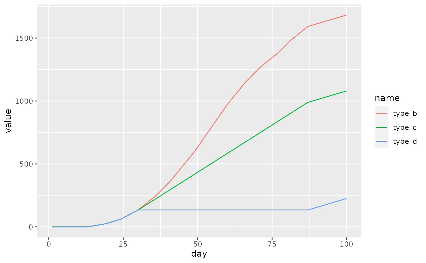

The above figure clearly shows that the selection of the calculation method (type) can make a large difference in the output values. Therefore, it is crucial to select the type and other parameters (tbase and tbase_max) that are appropriate for the studied phase in the plant or animal development.

References

Baskerville, G. L., and P. Emin. 1969. “Rapid Estimation of Heat Accumulation from Maximum and Minimum Temperatures.” Ecology 50 (3): 514–17. https://doi.org/10.2307/1933912.

Jakub Nowosad

2025-09-30

References