
library(raster)
# downloading the example data
temp_data_file = tempfile(fileext = ".tif")
download.file("https://github.com/Nowosad/ent_bp/raw/master/data/landscapes.tif",
              destfile = temp_data_file)
# read the example data
landscapes = brick(temp_data_file)Quantitative assessment of spatial patterns has been a keen interest of generations of spatial scientists and practitioners using spatial data. This post describes Information Theory-based metrics allowing for numerical description of spatial patterns. Each example is accompanied by an R code allowing for reproducing these results and encouraging to try these metrics on different data.
To learn more about this topic, read our open access article:
Nowosad, J., and T. F. Stepinski. (2019). Information Theory as a consistent framework for quantification and classification of landscape patterns. Landscape Ecology, DOI: 10.1007/s10980-019-00830-x
Example data
To reproduce the calculations in this blog post, you need to download the landscapes.tif file containing the example data.
The data can be visualized using the tmap package.
library(tmap)
tm_shape(landscapes) +
  tm_raster(palette = c("#FFFF64", "#006400", "#966400", "#BE9600"),
            style = "cat",
            title = "Land cover category",
            labels = c("Argiculture", "Forest", "Shrubland", "Grassland")) +
  tm_facets(free.scales = FALSE, nrow = 1) +
  tm_layout(panel.labels = 1:6, legend.outside.position = "bottom")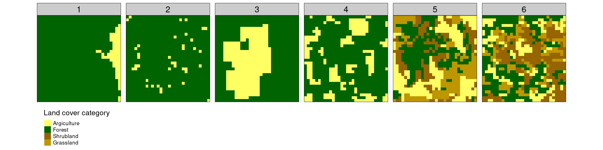
Let’s consider six fairly simple, but diverse examples:
- One dominating category and second spatially aggregated minor category
- One dominating category and second spatially disaggregated minor category
- One less dominating category and second spatially aggregated minor category
- One less dominating category and second spatially disaggregated minor category
- Four categories, where each one is spatially aggregated
- Four categories, where each one is spatially disaggregated
The example data represent different land cover categories; however, they could be any discrete values. Additionally, those cases are only a small subset of possible spatial arrangement, but the ideas presented below works for more and less complex cases.
Spatial representation
One of the ways to describe the above examples is to count a number of cells for each category (this metrics is known as a composition). However, this representation does not contain any information about the spatial distribution of the values. For example, let’s consider example data 1 and 2 – they both have a very similar number of cells for each category, but the spatial arrangement of the values is very different.
Another way to represent the above example is to calculate a co-occurrence matrix.1 It is created by counting all of the pairs of the adjacent cells in the data. As you will see below, this representation describes not only composition but also spatial configuration of the values.
The landscapemetrics package allows for calculating co-occurrence matrices using the get_adjacencies() function.
library(landscapemetrics)
get_adjacencies(landscapes)
$layer_1
1 2
1 200 50
2 50 3180
$layer_2
1 2
1 22 130
2 130 3198
$layer_3
1 2
1 1142 106
2 106 2126
$layer_4
1 2
1 546 304
2 304 2326
$layer_5
1 2 3 4
1 712 47 144 62
2 47 684 183 108
3 144 183 370 35
4 62 108 35 556
$layer_6
1 2 3 4
1 294 168 107 85
2 168 748 95 152
3 107 95 684 139
4 85 152 139 262The result for each example dataset is a matrix with a number of rows and columns equal to the number of unique categories in the dataset. For example data 1, 200 times cells of the first category are adjacent to other cells of this category, 3180 times cells of the second category are adjacent to other cells of this category, and 50 times cells of the first category are adjacent to cells of the second category. This representation shows that the second category dominates in the data (3180 pairs), but also that the cells from the first category are more often next to other cells of this category than a different one (200 vs. 50).
Information theory
The co-occurrence matrix representation is not only compact but also allows to calculate several metrics based on the information theory applied to bivariate random variable (x,y), where x is a category of a focus cell and y is category of a cell adjacent to it. This metrics are include marginal entropy, conditional entropy, joint entropy, mutual information, and relative mutual information.
Marginal entropy [H(x)]
The first metric, marginal entropy, represents a diversity (thematic complexity, composition) of spatial categories. It is calculated as the entropy of the marginal distribution. The lsm_l_ent() function allows for calculating marginal entropy. Its output gives a layer number (example data id), informs that the data is only of the landscape level, this metric abbreviation is ent, and finally it shows the resulting value.
mar_ent = lsm_l_ent(landscapes)
mar_ent
# A tibble: 6 × 6
layer level class id metric value
<int> <chr> <int> <int> <chr> <dbl>
1 1 landscape NA NA ent 0.373
2 2 landscape NA NA ent 0.259
3 3 landscape NA NA ent 0.942
4 4 landscape NA NA ent 0.802
5 5 landscape NA NA ent 1.98
6 6 landscape NA NA ent 1.95 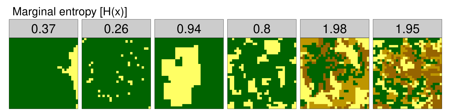
The resulting values indicate that the example datasets have different levels of thematic complexity. Example data 1 and 2 have one dominating category (low values of marginal entropy), while categories are more evenly distributed in example data 3 and 4 (medium values of marginal entropy). Example data 5 and 6 have the highest levels of thematic complexity due to the fact of having more unique, evenly distributed categories.
Conditional entropy [H(y|x)]
The second metric, conditional entropy, represents a configurational complexity (geometric intricacy) of a spatial pattern. If the value of conditional entropy is small, cells of one category are predominantly adjacent to only one category of cells. On the other hand, the high value of conditional entropy shows that cells of one category are adjacent to cells of many different categories. Conditional entropy can be calculated using the lsm_l_condent() function.
cond_ent = lsm_l_condent(landscapes)
cond_ent
# A tibble: 6 × 6
layer level class id metric value
<int> <chr> <int> <int> <chr> <dbl>
1 1 landscape NA NA condent 0.159
2 2 landscape NA NA condent 0.254
3 3 landscape NA NA condent 0.327
4 4 landscape NA NA condent 0.620
5 5 landscape NA NA condent 1.36
6 6 landscape NA NA condent 1.61 
The conditional entropy values are the smallest for example data 1, where most of the “green” cells are adjacent to other “green” ones, and the “yellow” cells are next to other “yellow” cells, and where one category (“green”) dominates the entire area. In example data 2, the proportion of categories is similar; however, the configuration of the cells is less organized and therefore the conditional entropy value is higher than in example data 1. For the next examples, the conditional entropy values grow with both categories proportions and their arrangement. This is due to the fact that the diversity of categories induces configurational complexity.
Joint entropy [H(x, y)]
The third metric, joint entropy, is an overall spatio-thematic complexity metric. It represents the uncertainty in determining a category of the focus cell and the category of the adjacent cell. In other words, it measures diversity of values in a co-occurrence matrix – the smaller the diversity, the larger the value of joint entropy. You can use the lsm_l_joinent() to calculate this metric.
join_ent = lsm_l_joinent(landscapes)
join_ent
# A tibble: 6 × 6
layer level class id metric value
<int> <chr> <int> <int> <chr> <dbl>
1 1 landscape NA NA joinent 0.532
2 2 landscape NA NA joinent 0.513
3 3 landscape NA NA joinent 1.27
4 4 landscape NA NA joinent 1.42
5 5 landscape NA NA joinent 3.34
6 6 landscape NA NA joinent 3.56 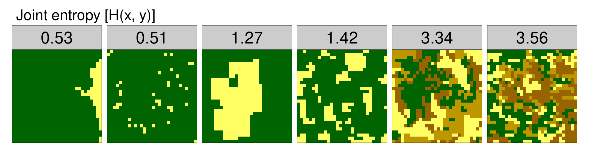
The values of joint entropy organize the example data from the most simple (example data 2) to the most complex (example data 6). However, joint entropy alone is not capable to sufficiently distinguish situations with spatially aggregated values (example data 1, 3, and 5) from situations that are spatially disaggregated (example data 2, 4, 6).
Mutual information [I(y,x)]
The fourth metric, mutual information, quantifies the information that one random variable (x) provides about another random variable (y). It tells how much easier is to predict a category of an adjacent cell if the category of the focus cell is known. Mutual information disambiguates landscape pattern types characterized by the same value of overall complexity. The lsm_l_mutinf() function calculates mutual information.
mut_inf = lsm_l_mutinf(landscapes)
mut_inf
# A tibble: 6 × 6
layer level class id metric value
<int> <chr> <int> <int> <chr> <dbl>
1 1 landscape NA NA mutinf 0.214
2 2 landscape NA NA mutinf 0.00527
3 3 landscape NA NA mutinf 0.614
4 4 landscape NA NA mutinf 0.182
5 5 landscape NA NA mutinf 0.627
6 6 landscape NA NA mutinf 0.337 
Larger values indicate that the cells of the same category are more aggregated, while the smaller values are an indication of disaggregation.
Relative mutual information [U]
Due to the spatial autocorrelation, the value of mutual information tends to grow with a diversity of the landscape (marginal entropy). To adjust this tendency, it is possible to calculate relative mutual information by dividing the mutual information by the marginal entropy. Relative mutual information always has a range between 0 and 1 and can be used to compare spatial data with different number and distribution of categories.
rel_mut_inf = lsm_l_mutinf(landscapes)$value / lsm_l_ent(landscapes)$value
rel_mut_inf
[1] 0.57389601 0.02036298 0.65250917 0.22678349 0.31603770 0.17301316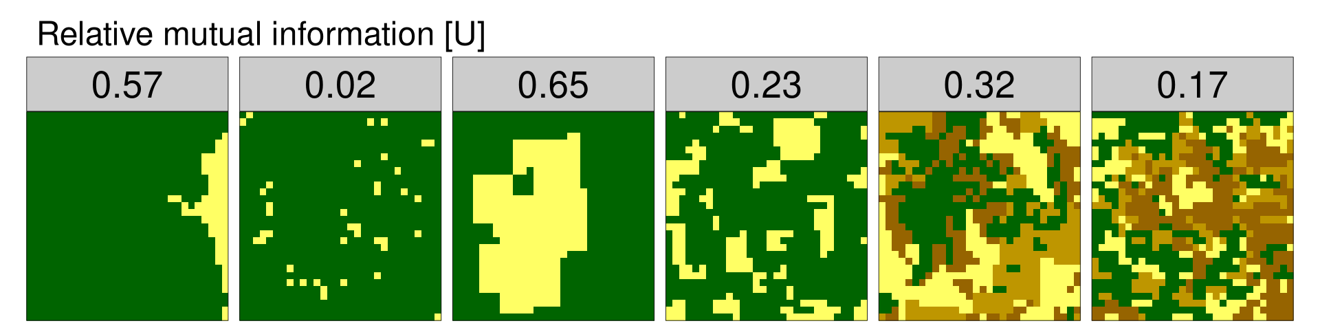
Relative mutual information for the example data orders them from the least aggregated (example data 2, 6), through those with medium aggregation (example data 4, 5), to the most aggregated (example data 1 and 2), without the influence of the number or distribution of categories.
Applications
The direct applications of the above metrics are ordering and classifying of spatial patterns. Each of the presented metrics can be used alone to order the spatial data according to a different property. For example, values of marginal entropy orders by the diversity of spatial categories, while values of relative mutual information orders by spatial aggregation. Two or more of the above metrics can be a basis for spatial classification, grouping similar spatial pattern together.
These basic applications can be further used for a myriad of practical purposes. For example, let’s consider spatial data representing a land cover. An area’s pattern is related to many environmental characteristics and processes, such as vegetation diversity, animal distribution, or water quality. Therefore, the possibility of a quantitative assessment of spatial patterns could enable a better understanding of this relationship, and allow for improvements in management and conservation of the environment.
Spatial patterns do exist in many other domains, including urban science, demography, agriculture, etc. Consequently, these metrics can be used to add new knowledge to these domains.
Summary
Information theory provides a framework for quantification of the spatial patterns. This includes several metrics based on the co-occurrence matrix, such as marginal entropy, conditional entropy, joint entropy, mutual information, and relative mutual information.
The landscapemetrics R package implements these metrics as the lsm_l_ent() (marginal entropy), lsm_l_condent() (conditional entropy), lsm_l_joinent() (joint entropy), and lsm_l_mutinf() (mutual information) functions. The function accepts raster data (in the form of Raster*, matrix, or stars objects) as an input. Additional parameters include cells adjacency type (4-connected or 8-connected), type of pairs considered (ordered and unordered), and the unit in which entropy is measured (logarithm to base 2, natural logarithm, and logarithm to base 10).
A complete demonstration of the spatial patterns quantification within the framework of the Information Theory is in the open access Landscape Ecology article. The article shows that one-dimensional parametrizations of patterns using the information theory based measures correspond to orderings, and two-dimensional parametrizations correspond to classifications. These findings are based on the dataset which contains a rich variety of land cover patterns. Different pattern metrics are compared, and the correlation coefficients between them are calculated. Finally, the article shows an example of how these concepts can be used for spatial patterns classifications by grouping similar patterns into distinct regions of the parameters space.
Footnotes
Another name for this representation is the adjacency matrix.↩︎
Reuse
Citation
BibTeX citation:
@online{nowosad2019,
  author = {Nowosad, Jakub},
  title = {Information Theory Provides a Consistent Framework for the
    Analysis of Spatial Patterns},
  date = {2019-06-25},
  url = {https://jakubnowosad.com/posts/2019-06-25-ent-bp1/},
  langid = {en}
}
For attribution, please cite this work as:
Nowosad, Jakub. 2019. “Information Theory Provides a Consistent
Framework for the Analysis of Spatial Patterns.” June 25. https://jakubnowosad.com/posts/2019-06-25-ent-bp1/.