
TLTR:
Spatial signatures are multi-value representations of the patterns that compress information about spatial composition and configuration. Spatial signatures can be directly compared using various distance measures.
Describing categorical rasters
A categorical raster shown below represents land cover data for some area. This area is mainly covered by forest, with some small patches of agriculture, grasslands, and water.
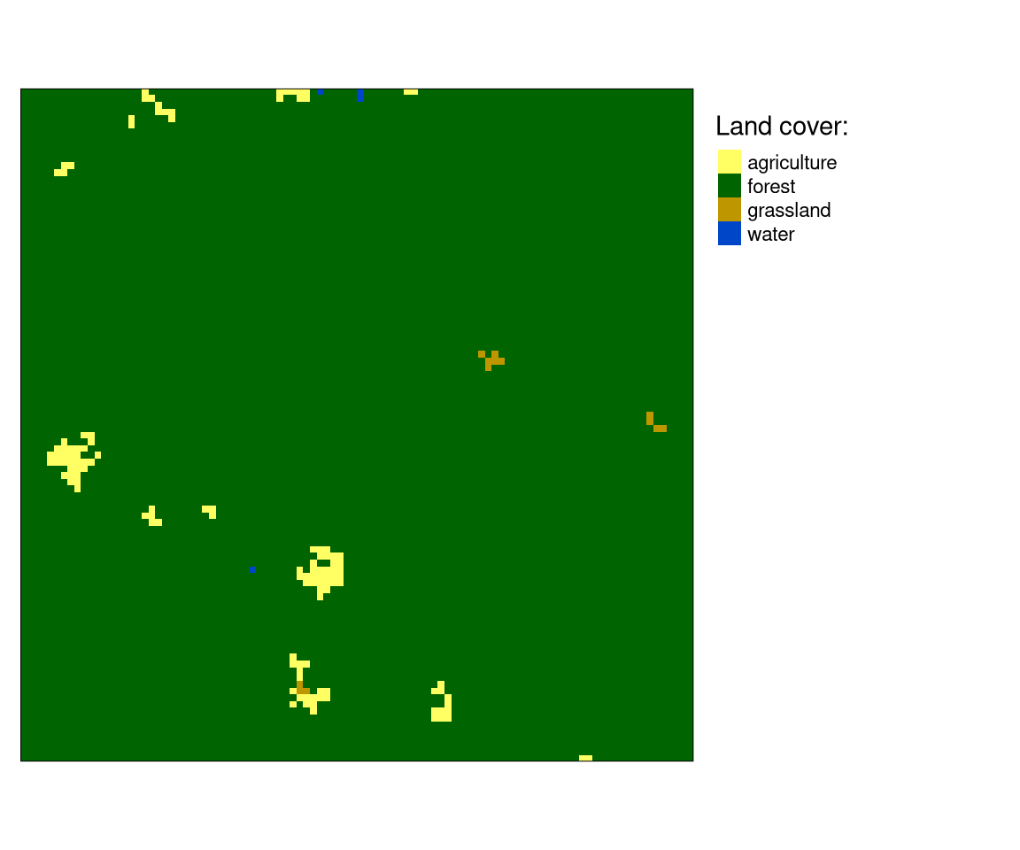
If we want to describe this area, we could start by measuring areas of different land cover categories. Then, we could know that forest cover about 0.986% and agriculture cover about 0.013%. We could also use landscape metrics to put a number on some property of this raster. Then, we would know that the entropy is 0.116, and relative mutual information is 0.3311.
This approach can be applied to many categorical rasters, as you can see below.
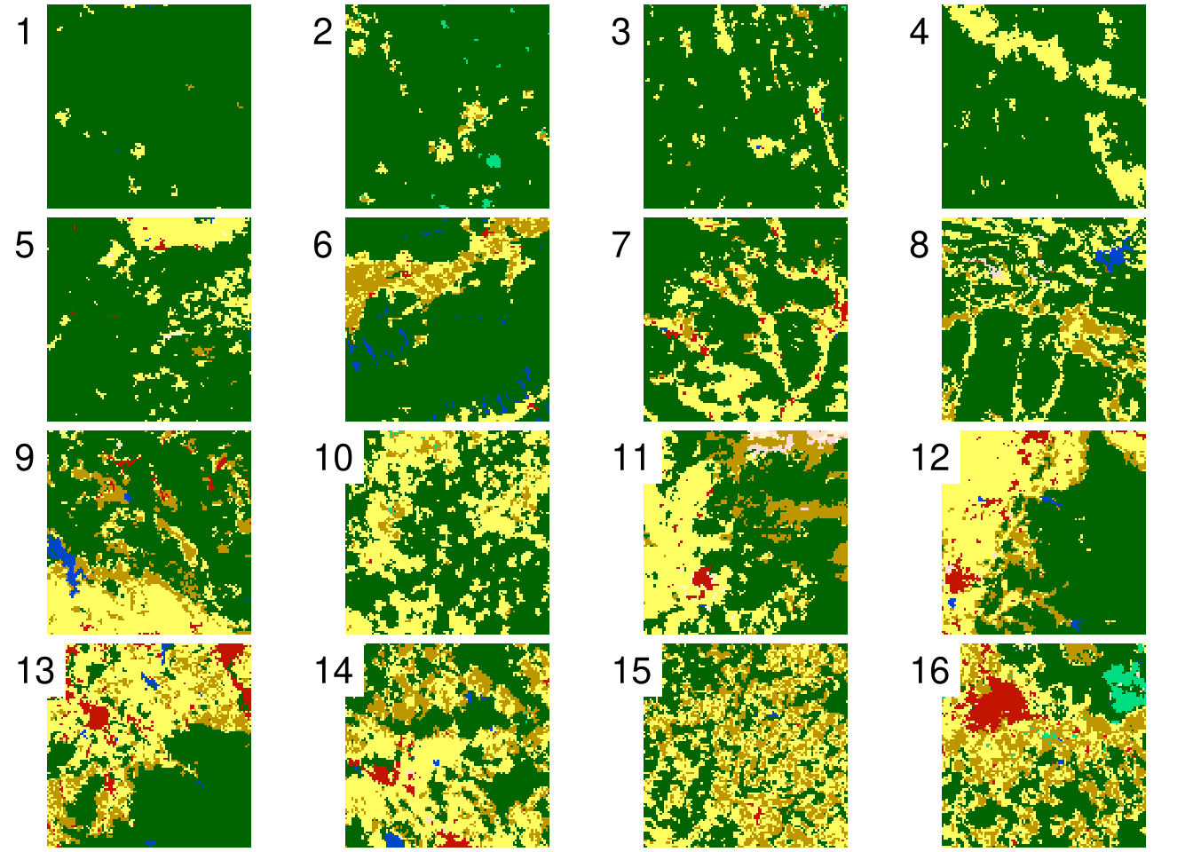
| id | 1 | 2 | 3 | 4 | 5 | 6 | 7 | 8 | 9 | 10 | 11 | 12 | 13 | 14 | 15 | 16 |
| ent | 0.12 | 0.45 | 0.53 | 0.63 | 0.75 | 1.16 | 1.16 | 1.28 | 1.53 | 1.2 | 1.65 | 1.6 | 1.74 | 1.72 | 1.6 | 2.02 |
| relmutinf | 0.33 | 0.39 | 0.34 | 0.52 | 0.44 | 0.51 | 0.39 | 0.33 | 0.42 | 0.36 | 0.5 | 0.58 | 0.43 | 0.34 | 0.2 | 0.38 |
| forest | 0.99 | 0.93 | 0.9 | 0.84 | 0.83 | 0.76 | 0.69 | 0.68 | 0.59 | 0.57 | 0.53 | 0.5 | 0.44 | 0.4 | 0.39 | 0.36 |
| agriculture | 0.01 | 0.05 | 0.08 | 0.16 | 0.16 | 0.12 | 0.25 | 0.23 | 0.24 | 0.39 | 0.3 | 0.36 | 0.36 | 0.39 | 0.36 | 0.3 |
Now, each rasters’ spatial properties are expressed by a vector of numbers representing its categories and selected landscape metrics.
Basic spatial signature
As I mentioned in my previous blog posts, we could represent categorical rasters with a large number of landscape metrics. However, many landscape metrics are highly correlated, and some of them depend on the resolution of the input data and the size of the study area.
An alternative approach is to derive a multi-value representation of the raster that compress information about its spatial composition and configuration. One of such representations is a co-occurrence matrix (coma).
The coma representation is calculated by moving through each cell, looking at its value, and counting how many neighbors of each class our central cell has. For example, the co-occurrence matrix below shows that the forest category cells are 38,778 times adjacent to other cells of this category, 218 times to the cells of the agriculture category, and four times to the cells of the grassland category, and so on.
| agriculture | forest | grassland | water | |
|---|---|---|---|---|
| agriculture | 272 | 218 | 4 | 0 |
| forest | 218 | 38778 | 32 | 12 |
| grassland | 4 | 32 | 16 | 0 |
| water | 0 | 12 | 0 | 2 |
Importantly, this signature contains information about the categories and their shares (composition), and also the spatial relation between categories (configuration).
The co-occurrence matrix (coma) representation is two-dimensional, with values of categories in row and columns. It can be converted into a one-dimensional representation called a co-occurrence vector (cove).
| 272 | 218 | 4 | 0 | 218 | 38778 | 32 | 12 | 4 | 32 | 16 | 0 | 0 | 12 | 0 | 2 |
As you can see, some elements of this vector represent the same relations. For example, the first value of 4 shows the relation between grassland and agriculture, and the second value of 4 represents the relation between agriculture and grassland. We can simplify the above vector by counting all relations only once2:
| 136 | 218 | 19389 | 4 | 32 | 8 | 0 | 12 | 0 | 1 |
This vector can be further transformed to have its values to sum up to one. The output vector is called the normalized co-occurrence vector.
| 0.0069 | 0.011 | 0.9792 | 0.0002 | 0.0016 | 0.0004 | 0 | 0.0006 | 0 | 0.0001 |
The role of normalization is to create a probability function, and thus be able to compare categorical rasters of different sizes using mathematical distance measures.
Measuring similarity between patterns
Let’s consider two rasters below. We want to know how similar they are to each other.
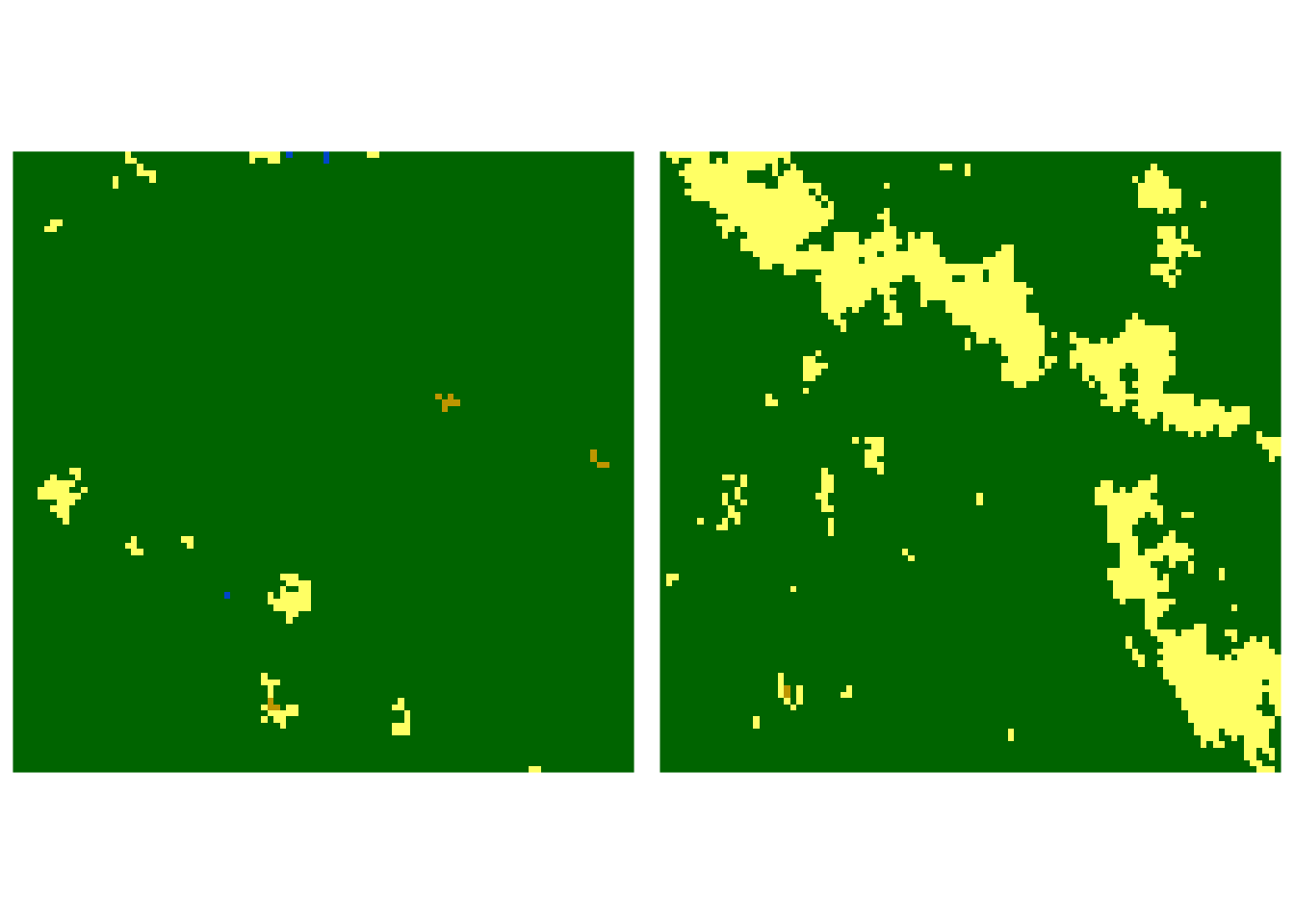
To answer this question, we need to perform three steps:
- calculate a normalized co-occurrence vector for the first raster,
- calculate a normalized co-occurrence vector for the second raster,
- calculate a numerical distance between these two signatures.
Normalized co-occurrence vector for the first raster is:
| 0.0069 | 0.011 | 0.9792 | 0.0002 | 0.0016 | 0.0004 | 0 | 0.0006 | 0 | 0.0001 |
Normalized co-occurrence vector for the second raster is:
| 0.1282 | 0.0609 | 0.8105 | 0.0002 | 0.0002 | 0.0001 | 0 | 0 | 0 | 0 |
A large number of possible distance measures between probability functions exists3. In this example, we use the Jenson-Shannon distance.
$$ JSD(A, B) = H(\frac{A + B}{2}) - \frac{1}{2}[H(A) + H(B)] $$
It takes two probability functions (spatial signatures in our case) A and B, and calculates entropy values (H). The Jenson-Shannon distance is a value between 0 and 1, where 0 means that two probability functions are identical, and 1 means that they have nothing in common.
Jensen-Shannon distance between our two rasters is 0.068, suggesting that their spatial composition and configuration are fairly similar, but not identical. Now, let’s consider two rasters that are visually very different. One is covered mostly by forest, while the second one is mostly a mosaic of forests, agricultural areas, and grasslands.
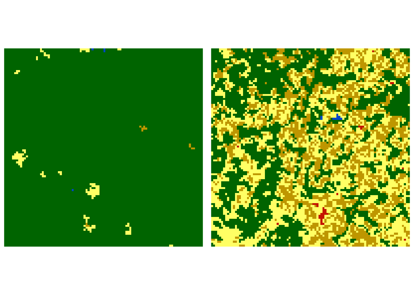
Normalized co-occurrence vector for the first raster is:
| 0.0069 | 0.011 | 0.9792 | 0.0002 | 0.0016 | 0.0004 | 0 | 0 | 0 | 0 | 0 | 0.0006 | 0 | 0 | 0.0001 |
Normalized co-occurrence vector for the second raster is:
| 0.2033 | 0.1335 | 0.2944 | 0.1747 | 0.0562 | 0.1307 | 0.0035 | 0.0002 | 0.0004 | 0.0015 | 0.0007 | 0.0005 | 0 | 0 | 0.0005 |
The Jensen-Shannon distance between this pair of rasters is 0.444, indicating that two rasters are fairly different4.
Calculating spatial signatures for many areas allows us to find the most similar rasters, describe changes between rasters, or group (cluster) rasters with similar spatial patterns.
Other spatial signatures
The co-occurrence matrix (coma) is suitable to represent pattern of a single categorical variable. There are, however, other spatial signatures aimed to describe spatial patterns of multi-variable cases.
A weighted co-occurrence matrix (wecoma) representation
Let’s consider a situation, in which we have two rasters: one with categories, and one with weights. So, now we have not only a category of each cell, but also its intensity.
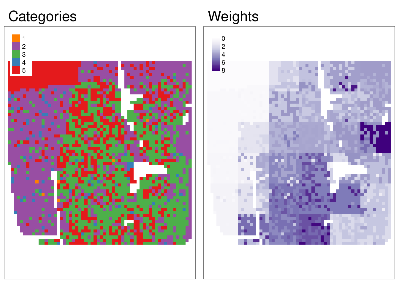
Regular co-occurrence matrix (coma) based just on a categorical raster looks the following:
| 1 | 2 | 3 | 4 | 5 | |
|---|---|---|---|---|---|
| 1 | 0 | 4 | 5 | 0 | 1 |
| 2 | 4 | 1652 | 493 | 86 | 316 |
| 3 | 5 | 493 | 1148 | 38 | 509 |
| 4 | 0 | 86 | 38 | 6 | 14 |
| 5 | 1 | 316 | 509 | 14 | 818 |
It represents a spatial pattern of the categories, however, it completely omits the secondary information about the weight of each raster cell. To utilize the secondary information, a weighted co-occurrence matrix (wecoma) was developed. It is a modification of the co-occurrence matrix, in which each adjacency contributes to the output based on the values from the weight raster. The contributed value is calculated as the average of the weights in the two adjacent cells.
| 1 | 2 | 3 | 4 | 5 | |
|---|---|---|---|---|---|
| 1 | 0.00 | 7.08 | 15.42 | 0.00 | 2.18 |
| 2 | 7.08 | 3513.53 | 1723.24 | 92.45 | 923.97 |
| 3 | 15.42 | 1723.24 | 4524.03 | 113.75 | 2029.07 |
| 4 | 0.00 | 92.45 | 113.75 | 3.72 | 36.37 |
| 5 | 2.18 | 923.97 | 2029.07 | 36.37 | 1574.14 |
As you can see above, the weighted co-occurrence matrix differs from regular coma.
Similarly to the previous case, we can also convert wecoma into a one-dimensional normalized representation now called a weighted co-occurrence vector (wecove):
| 0 | 0.0007 | 0.1802 | 0.0016 | 0.1767 | 0.232 | 0 | 0.0095 | 0.0117 | 0.0002 | 0.0002 | 0.0948 | 0.2081 | 0.0037 | 0.0807 |
You can also see the weighted co-occurrence matrix (wecoma) concept, there described as an exposure matrix, in action in the vignettes of the raceland package.
An integrated co-occurrence matrix (incoma) representation
Another situation would be when we have two or more categorical raster variables. For example, let’s consider one raster with land cover categories and one with landform classes.
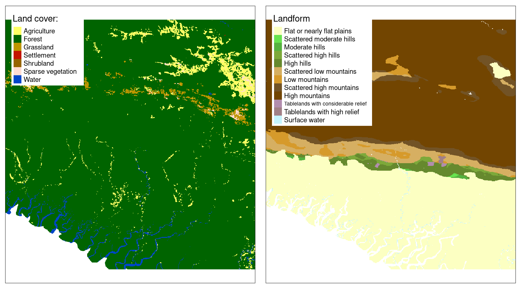
The question here is how to create a signature that incorporates spatial patterns of both land cover and landform data? The apparent solution would be to create a new raster with the joint-distribution of class labels. For example, if agriculture is represented as 1 in the first raster and flat plains are represented as 1 in the second raster, then a value of 101 would represent agriculture on a flat plain in a new raster. Next, we could just calculate a regular co-occurrence matrix. However, this approach is not recommended - by creating joint labels in this example data, we would end up with 84 categories, and therefore with a co-occurrence matrix of 84 by 84. Large signatures not only occupy more storage but also are harder to meaningfuly compare.
An alternative approach is to use an integrated co-occurrence matrix (incoma). It consists of co-occurrence matrices (coma) and co-located co-occurrence matrices (cocoma). In the co-occurrence matrix, we only use one raster and count adjacent categories of each cell. The co-located co-occurrence matrix, on the other hand, uses two rasters and counts neighbors in the second raster for each cell in the first raster.
The incoma representation for two rasters consists of four sectors (see an example below):
- A co-occurrence matrix for the first raster.
- A co-located co-occurrence matrix between the first raster and the second raster. It is between the first and third column and the third and fourth row.
- A co-located co-occurrence matrix between the second and the first raster.
- A co-occurrence matrix for the second raster.
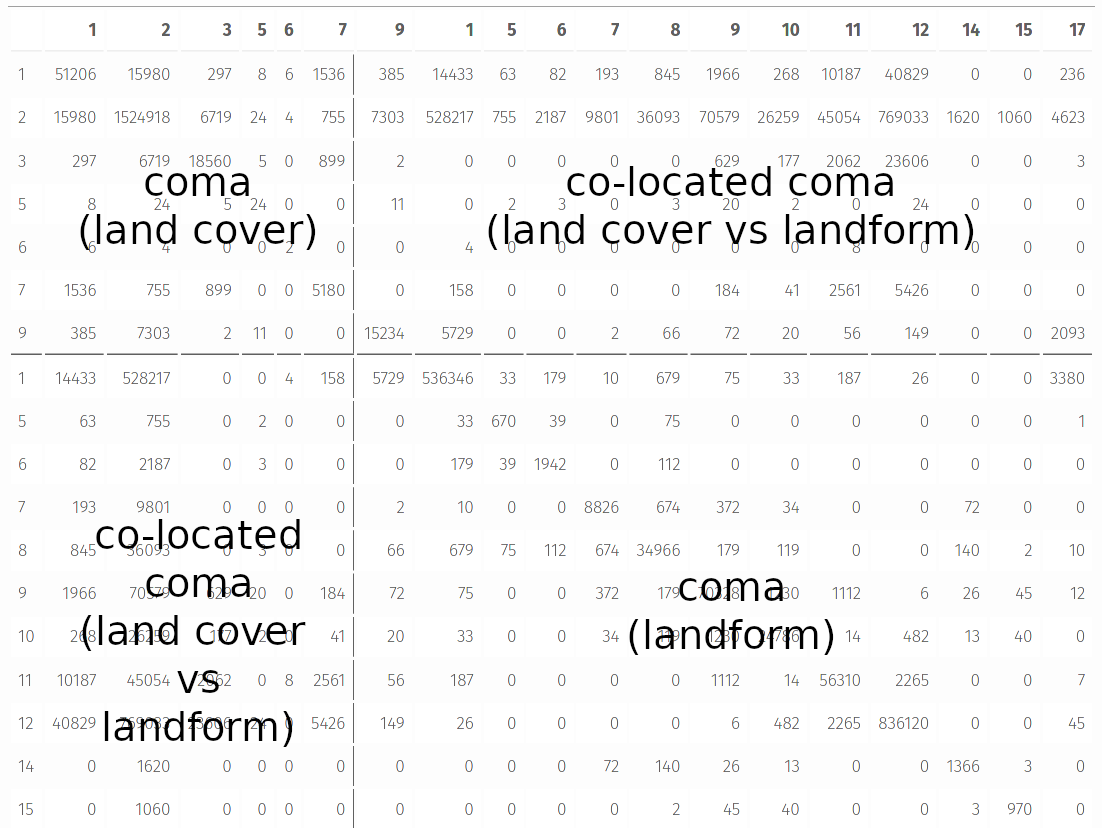
Similar to the previous signatures, it is possible to convert incoma to its 1D normalized representation called an integrated co-occurrence vector (incove).
Summary
Spatial signatures allow to store compressed information about spatial patterns of many types of data. It includes a co-occurrence matrix (coma) for regular categorical rasters, a weighted co-occurrence matrix (wecoma) for categorical rasters with related intensity rasters, and an integrated co-occurrence matrix (incoma) for two or more categorical rasters. A spatial signature can be represented by 1D vectors and compared using a large number of distance measures.
To learn more how different spatial signatures can be calculated read the Types of spatial patterns’ signatures, A co-occurrence matrix (coma) representation, A weighted co-occurrence matrix (wecoma) representation, and An integrated co-occurrence matrix (incoma) representation vignettes.
Footnotes
See the Information theory provides a consistent framework for the analysis of spatial patterns blog post.↩︎
It also means dividing the diagonal by two.↩︎
Read https://users.uom.gr/~kouiruki/sung.pdf for a comprehensive review of distance measures.↩︎
Larger values of the Jensen-Shannon distance could occur when two rasters have different categories↩︎
Reuse
Citation
@online{nowosad2021,
  author = {Nowosad, Jakub},
  title = {Describing Categorical Rasters with Spatial Signatures},
  date = {2021-02-10},
  url = {https://jakubnowosad.com/posts/2021-02-10-motif-bp2/},
  langid = {en}
}
