
![]()
TLTR:
Clustering similar spatial patterns requires one or more raster datasets for the same area. Input data is divided into many sub-areas, and spatial signatures are derived for each sub-area. Next, distances between signatures for each sub-area are calculated and stored in a distance matrix. The distance matrix can be used to create clusters of similar spatial patterns. Quality of clusters can be assessed visually using a pattern mosaic or with dedicated quality metrics.
Spatial data
To reproduce the calculations in the following post, you need to download all of relevant datasets using the code below:
library(osfr)
dir.create("data")
osf_retrieve_node("xykzv") %>%
        osf_ls_files(n_max = Inf) %>%
        osf_download(path = "data",
                     conflicts = "overwrite")
You should also attach the following packages:
library(sf)
library(stars)
library(motif)
library(tmap)
library(dplyr)
library(readr)
Land cover and landforms in Africa
The data/land_cover.tif contains land cover data and data/landform.tif is landform data for Africa. Both are single categorical rasters of the same extent and the same resolution (300 meters) that can be read into R using the read_stars() function.
lc = read_stars("data/land_cover.tif")
lf = read_stars("data/landform.tif")
Additionally, the data/lc_palette.csv file contains information about colors and labels of each land cover category, and data/lf_palette.csv stores information about colors and labels of each landform class.
lc_palette_df = read_csv("data/lc_palette.csv")
lf_palette_df = read_csv("data/lf_palette.csv")
names(lc_palette_df$color) = lc_palette_df$value
names(lf_palette_df$color) = lf_palette_df$value
Both datasets can be visualized with tmap.
tm_lc = tm_shape(lc) +
        tm_raster(style = "cat",
                  palette = lc_palette_df$color,
                  labels = lc_palette_df$label,
                  title = "Land cover:") +
        tm_layout(legend.position = c("LEFT", "BOTTOM"))
tm_lc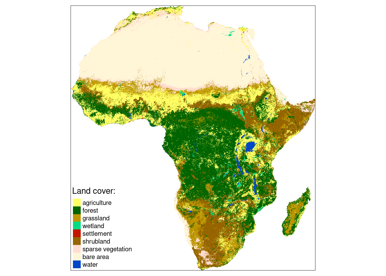
tm_lf = tm_shape(lf) +
        tm_raster(style = "cat",
                  palette = lf_palette_df$color,
                  labels = lf_palette_df$label,
                  title = "Landform:") +
        tm_layout(legend.outside = TRUE)
tm_lf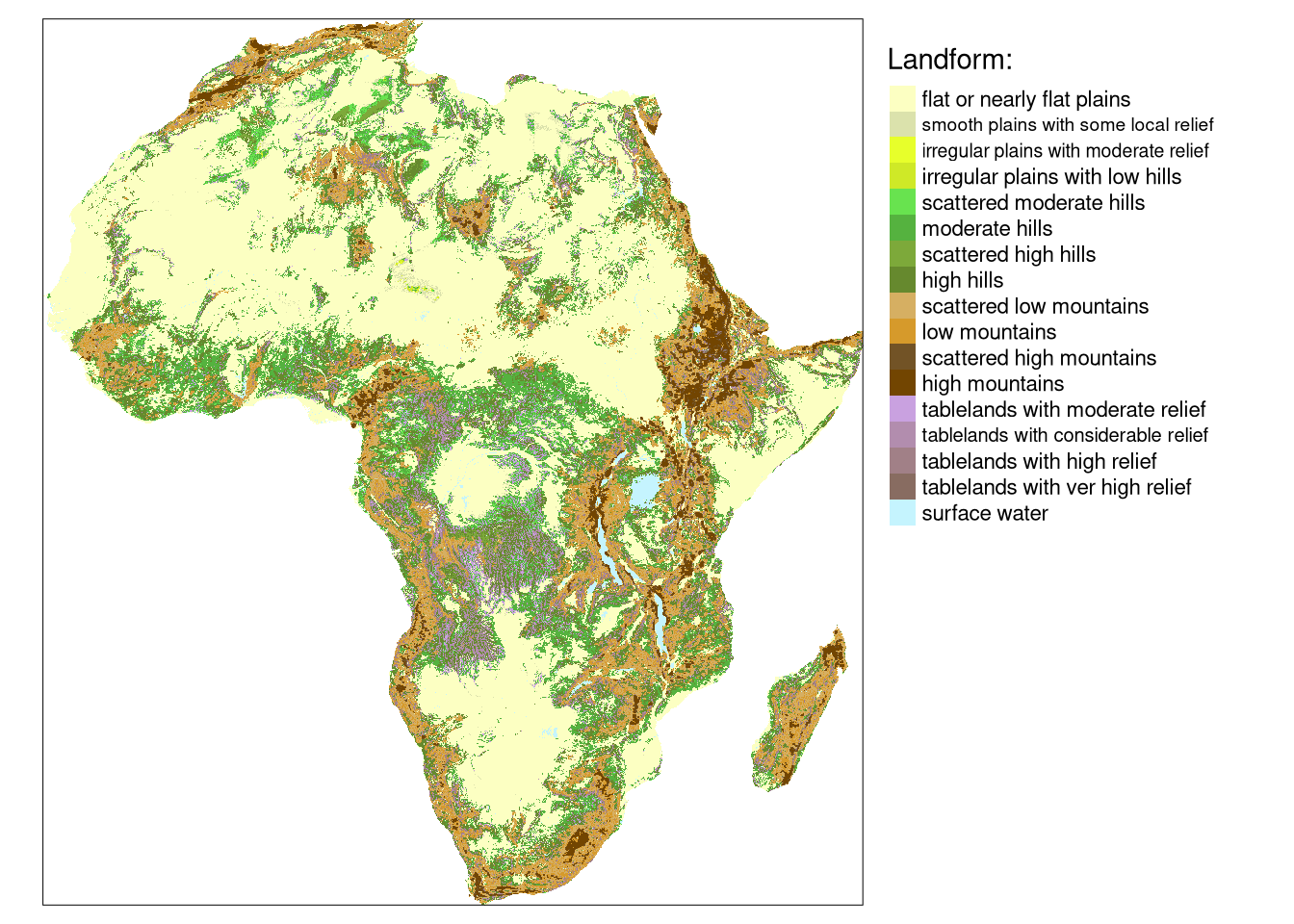
We can combine these two datasets together with the c() function.
eco_data = c(lc, lf)The problem now is how to find clusters of similar spatial patterns of both land cover categories and landform classes.
Clustering spatial patterns
The basic step in clustering spatial patterns is to calculate a proper signature for each spatial window using the lsp_signature() function. Here, we use the integrated co-occurrence vector (type = "cove") representation. In this example, we use a window of 300 cells by 300 cells (window = 300). This means that our search scale will be 90 km (300 cells x data resolution) - resulting in dividing the whole area into about 7,500 regular rectangles of 90 by 90 kilometers.
This operation could take a few minutes.
eco_signature = lsp_signature(eco_data,
                              type = "incove",
                              window = 300)
The output, eco_signature contains numerical representation for each 90 by 90 km area. Notice that it has 3,838 rows (not 7,500) - this is due to removing areas with a large number of missing values before calculations1.
Distance matrix
Next, we can calculate the distance (dissimilarity) between patterns of each area. This can be done with the lsp_to_dist() function, where we must provide the output of lsp_signature() and a distance measure used (dist_fun = "jensen-shannon"). This operation also could take a few minutes.
eco_dist = lsp_to_dist(eco_signature, dist_fun = "jensen-shannon")The output, eco_dist, is of a dist class, where small values show that two areas have a similar joint spatial pattern of land cover categories and landform classes.
class(eco_dist)[1] "dist"Hierarchical clustering
Objects of class dist can be used by many existing R functions for clustering. It includes different approaches of hierarchical clustering (hclust(), cluster::agnes(), cluster::diana()) or fuzzy clustering (cluster::fanny()). In the below example, we use hierarchical clustering using hclust(), which expects a distance matrix as the first argument and a linkage method as the second one. Here, we use the Ward’s minimum variance method (method = "ward.D2") that minimizes the total within-cluster variance.
eco_hclust = hclust(eco_dist, method = "ward.D2")
plot(eco_hclust)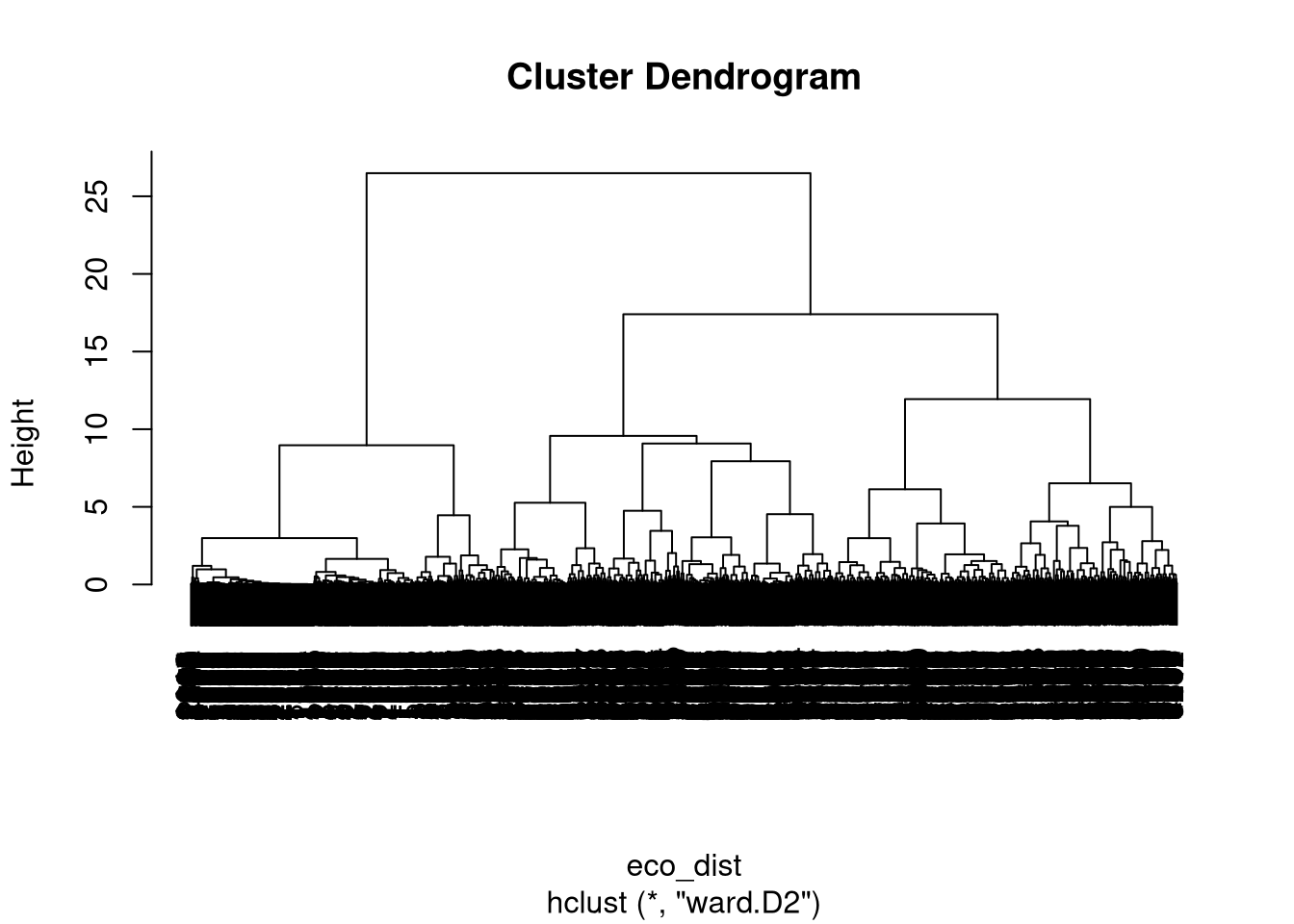
Graphical representation of the hierarchical clustering is called a dendrogram, and based on the obtained dendrogram, we can divide our local landscapes into a specified number of groups using cutree(). In this example, we use eight classes (k = 8) to create a fairly small number of clusters to showcase the presented methodology.
clusters = cutree(eco_hclust, k = 8)However, a decision about the number of clusters in real-life cases should be based on the goal of the research.
Clustering results
The lsp_add_clusters function adds: a column clust with a cluster number to each area, and converts the result to an sf object.
eco_grid_sf = lsp_add_clusters(eco_signature,
                               clusters)
The clustering results can be further visualized using tmap.
tm_clu = tm_shape(eco_grid_sf) +
        tm_polygons("clust", style = "cat", palette = "Set2", title = "Cluster:") +
        tm_layout(legend.position = c("LEFT", "BOTTOM"))
tm_clu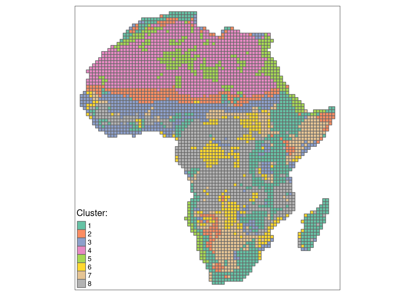
Most clusters form continuous regions, so we could merge areas of the same clusters into larger polygons.
eco_grid_sf2 = eco_grid_sf %>%
        dplyr::group_by(clust) %>%
        dplyr::summarize()
The output polygons can then be superimposed on maps of land cover categories and landform classes.
tm_shape(eco_data) +
                tm_raster(style = "cat",
                          palette = list(lc_palette_df$color, lf_palette_df$color)) +
  tm_facets(ncol = 2) +
  tm_shape(eco_grid_sf2) +
  tm_borders(col = "black") +
  tm_layout(legend.show = FALSE,
            title.position = c("LEFT", "TOP"))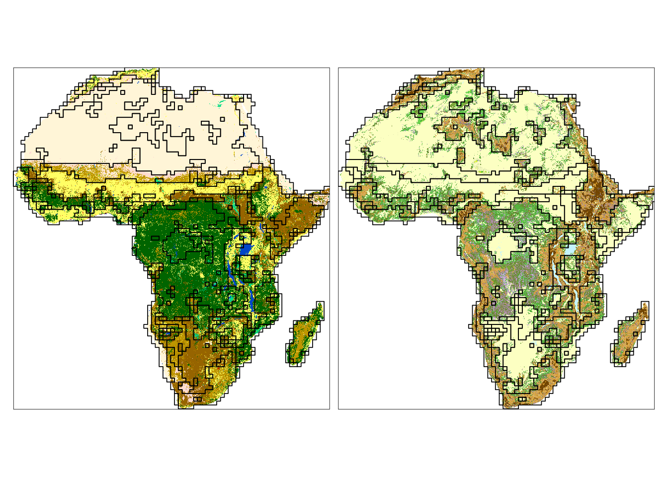
We can see that many borders (black lines) contain areas with both land cover or landform patterns distinct from their neighbors. Some clusters are also only distinct for one variable (e.g., look at Sahara on the land cover map).
Clustering quality
We can also calculate the quality of the clusters with the lsp_add_quality() function. It requires an output of lsp_add_clusters() and an output of lsp_to_dist(), and adds three new variables: inhomogeneity, distinction, and quality.
eco_grid_sfq = lsp_add_quality(eco_grid_sf, eco_dist, type = "cluster")Inhomogeneity (inhomogeneity) measures a degree of mutual distance between all objects in a cluster. This value is between 0 and 1, where the small value indicates that all objects in the cluster represent consistent patterns, so the cluster is pattern-homogeneous. Distinction (distinction) is an average distance between the focus cluster and all the other clusters. This value is between 0 and 1, where the large value indicates that the cluster stands out from the rest of the clusters. Overall quality (quality) is calculated as 1 - (inhomogeneity / distinction). This value is also between 0 and 1, where increased values indicate better quality of clustering.
We can create a summary of each clusters’ quality using the code below.
eco_grid_sfq2 = eco_grid_sfq %>%
        group_by(clust) %>%
        summarise(inhomogeneity = mean(inhomogeneity),
                  distinction = mean(distinction),
quality = mean(quality))| clust | inhomogeneity | distinction | quality |
|---|---|---|---|
| 1 | 0.5064706 | 0.7724361 | 0.3443204 |
| 2 | 0.4038704 | 0.7023297 | 0.4249561 |
| 3 | 0.3377875 | 0.7065250 | 0.5219029 |
| 4 | 0.1161293 | 0.7921515 | 0.8534002 |
| 5 | 0.3043422 | 0.7366735 | 0.5868696 |
| 6 | 0.2774136 | 0.6849140 | 0.5949657 |
| 7 | 0.2926504 | 0.7149212 | 0.5906537 |
| 8 | 0.3486704 | 0.7579511 | 0.5399830 |
The created clusters show a different degree of quality metrics. The fourth cluster has the lowest inhomogeneity and the largest distinction, and therefore the best quality. The first cluster has the most inhomogeneous patterns, and while its distinction from other clusters is relatively large, its overall quality is the worst.
tm_inh = tm_shape(eco_grid_sfq2) +
        tm_polygons("inhomogeneity", style = "cont", palette = "magma")

tm_iso = tm_shape(eco_grid_sfq2) +
        tm_polygons("distinction", style = "cont", palette = "-inferno")

tm_qua = tm_shape(eco_grid_sfq2) +
        tm_polygons("quality", style = "cont", palette = "Greens")

tm_cluster3 = tmap_arrange(tm_clu, tm_qua, tm_inh, tm_iso, ncol = 2)
tm_cluster3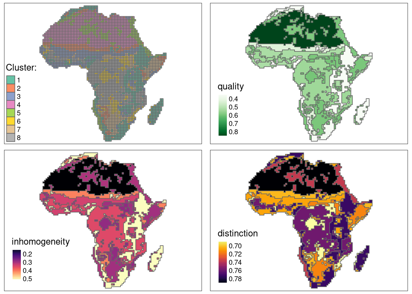
Understanding clusters
Inhomogeneity can also be assessed visually with a pattern mosaic. Pattern mosaic is an artificial rearrangement of a subset of randomly selected areas belonging to a given cluster.
Using the code below, we randomly selected 100 areas for each cluster. It could take a few minutes.
eco_grid_sample = eco_grid_sf %>%
  filter(na_prop == 0) %>%
  group_by(clust) %>%
  slice_sample(n = 100)
Next, we can extract a raster for each selected area with the lsp_add_examples() function.
eco_grid_examples = lsp_add_examples(eco_grid_sample, eco_data)Finally, we can use the lsp_mosaic() function, which creates raster mosaics by rearranging spatial data for sample areas. Note that this function is still experimental and can change in the future.
eco_mosaic = lsp_mosaic(eco_grid_examples)The output is a stars object with the third dimension (clust) representing clusters, from which we can use slice() to extract a raster mosaic for a selected cluster. For example, the raster mosaic for fourth cluster looks like this:
eco_mosaic_c4 = slice(eco_mosaic, clust, 4)

tm_shape(eco_mosaic_c4) +
  tm_raster(style = "cat",
            palette = list(lc_palette_df$color, lf_palette_df$color)) +
  tm_facets(ncol = 2) +
  tm_layout(legend.show = FALSE)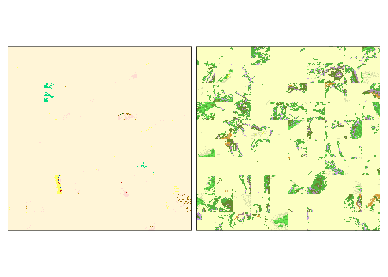
We can see that the land cover patterns for this cluster are very simple and homogeneous. The landform patterns are slightly more complex and less homogeneous.
And the raster mosaic for first cluster is:
eco_mosaic_c1 = slice(eco_mosaic, clust, 1)

tm_shape(eco_mosaic_c1) +
  tm_raster(style = "cat",
            palette = list(lc_palette_df$color, lf_palette_df$color)) +
  tm_facets(ncol = 2) +
  tm_layout(legend.show = FALSE)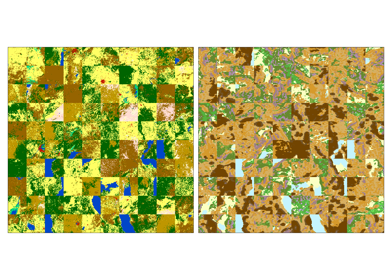
Patterns of both variables in this cluster are more complex and heterogeneous. This result could suggest that additional clusters could be necessary to distinguish some spatial patterns.
Summary
The pattern-based clustering allows for grouping areas with similar spatial patterns. The above example shows the search based on two-variable raster data (land cover and landform), but by using a different spatial signature, it can be performed on a single variable raster as well. R code for the pattern-based clustering can be found here, with other examples described in the Spatial patterns’ clustering vignette.
Footnotes
See the
thresholdargument for more details.↩︎
Reuse
Citation
BibTeX citation:
@online{nowosad2021,
  author = {Nowosad, Jakub},
  title = {Clustering Similar Spatial Patterns},
  date = {2021-03-03},
  url = {https://jakubnowosad.com/posts/2021-03-03-motif-bp5/},
  langid = {en}
}
For attribution, please cite this work as:
Nowosad, Jakub. 2021. “Clustering Similar Spatial
Patterns.” March 3. https://jakubnowosad.com/posts/2021-03-03-motif-bp5/.