library(supercells)
library(terra)
library(sf)
library(regional)
library(tmap)
flc = rast("/vsicurl/https://github.com/Nowosad/supercells-examples/blob/main/raw-data/all_ned.tif?raw=true")Segmentation is a process of partitioning space into smaller segments. For example, imagine looking at your family photo and trying to distinct individual people. Similarly, we can look at a satellite image (in RGB colors) with the goal of delineating where are the buildings, fields, roads, etc. In geography, segmentation can also be associated with regionalization. Here, our goal is not to detect objects (e.g., people or buildings) but rather areas with similar properties.
Segmentation/regionalization methods should minimize internal inhomogeneity and maximize external isolation. First, each segment (you can think of them as polygons) should contain similar values.1 For example, let’s consider two segments representing two different roofs. One roof is entirely covered by red tiles, while the roof of second one looks like a chessboard with red and brown tiles. Both of the segments are homogeneous, however, the latter is more complex than the former. Second segmentation property is the maximization of external isolation. This means that any given segment is different from its neighbors as much as possible.
Segmentation is an optimization problem – trying and testing all of possible segments borders and their properties may take a very long time, even for relatively small data. For that reason, some heuristics need to be used. One way to improve the output and reduce the time/processing cost of segmentation is to perform a preprocessing stage with superpixels.
Superpixels
The main idea of superpixels is to create groupings of adjacent cells that share common characteristics. This process often results in an over-segmentation – this is a situation when our segments (superpixels) are internally homogeneous, but not always very different from their neighbors.
Superpixels are used for two main reasons:
- Pixels are not natural entities. They are rather a consequence of the discrete representation of data. For example, depending on the data resolution, our roofs from the previous example can consist of 20 pixels or be just a fraction of one pixel.
- Superpixels, as groupings of adjacent cells, reduce the dimensionality of the data making further segmentation tasks easier. For example, we may end up with 5,000 superpixels, instead of 150,000 original pixels.
SLIC algorithm
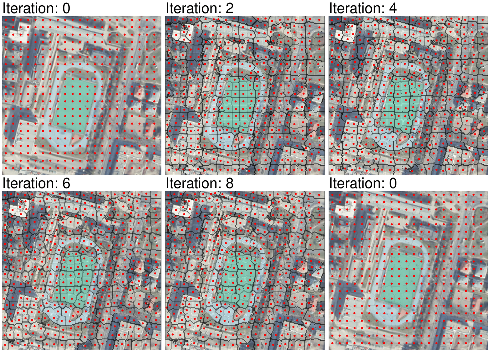
Many superpixels algorithms have been developed; see Stutz et al. (2018). The SLIC algorithm (Achanta et al. 2012) is one of the most often used superpixel algorithms due to its simplicity, accuracy, and low computational cost. It starts with cluster centers spaced by the interval of \(S\). Each cell is assigned to the nearest cluster center, and the distance \(D\) is calculated between the cluster centers and cells in the \(2S×2S\) region. Afterward, new cluster centers (centroids) are updated for the new superpixels, and their color values are the average of all the cells belonging to the given superpixel. The SLIC algorithm works iteratively, repeating the above process until it reaches the expected number of iterations.

The distance \(D\) is calculated as:
\[ D = \sqrt{\left(\frac{d_c}{m}\right)^2 + \left(\frac{d_s}{S}\right)^2} \]
where \(d_c\) is the color (spectral) distance, \(m\) is the compactness parameter, \(d_s\) is the spatial (Euclidean) distance, and \(S\) is the interval between the initial cluster centers.
Typical workflow for the original SLIC algorithm is to convert RGB image into the LAB color space and then use it to create superpixels. In that case, the distance \(D\) depends on (a) the Euclidean spatial distance between a cell and a superpixel centroid and (b) the Euclidean color distance between a cell’s LAB values and a superpixel centroid average LAB values. As originally implemented by its authors, the SLIC algorithm has the RGB image hard-wired as input data. Thus, its geospatial applications remain restricted to images, RGB, multispectral, or hyperspectral.
SLIC extension
In Nowosad and Stepinski (2022), we propose an extension of SLIC that can be applied to non-imagery geospatial rasters. This includes rasters that carry:
- Pattern information (co-occurrence matrices)
- Compositional information (histograms)
- Time-series information (ordered sequences)
- Other forms of information for which the use of Euclidean distance may not be justified2
The extended SLIC allows using any distance measure to calculate the semantic distance – \(dc\) can be replaced with any distance/dissimilarity measure. We implemented the above idea as an R package {supercells}. Note that we decided to use the supercells name (instead of superpixels) to highlight that the method can be applied to various spatial raster data. The package installation instructions can be found at https://jakubnowosad.com/supercells/.
Example
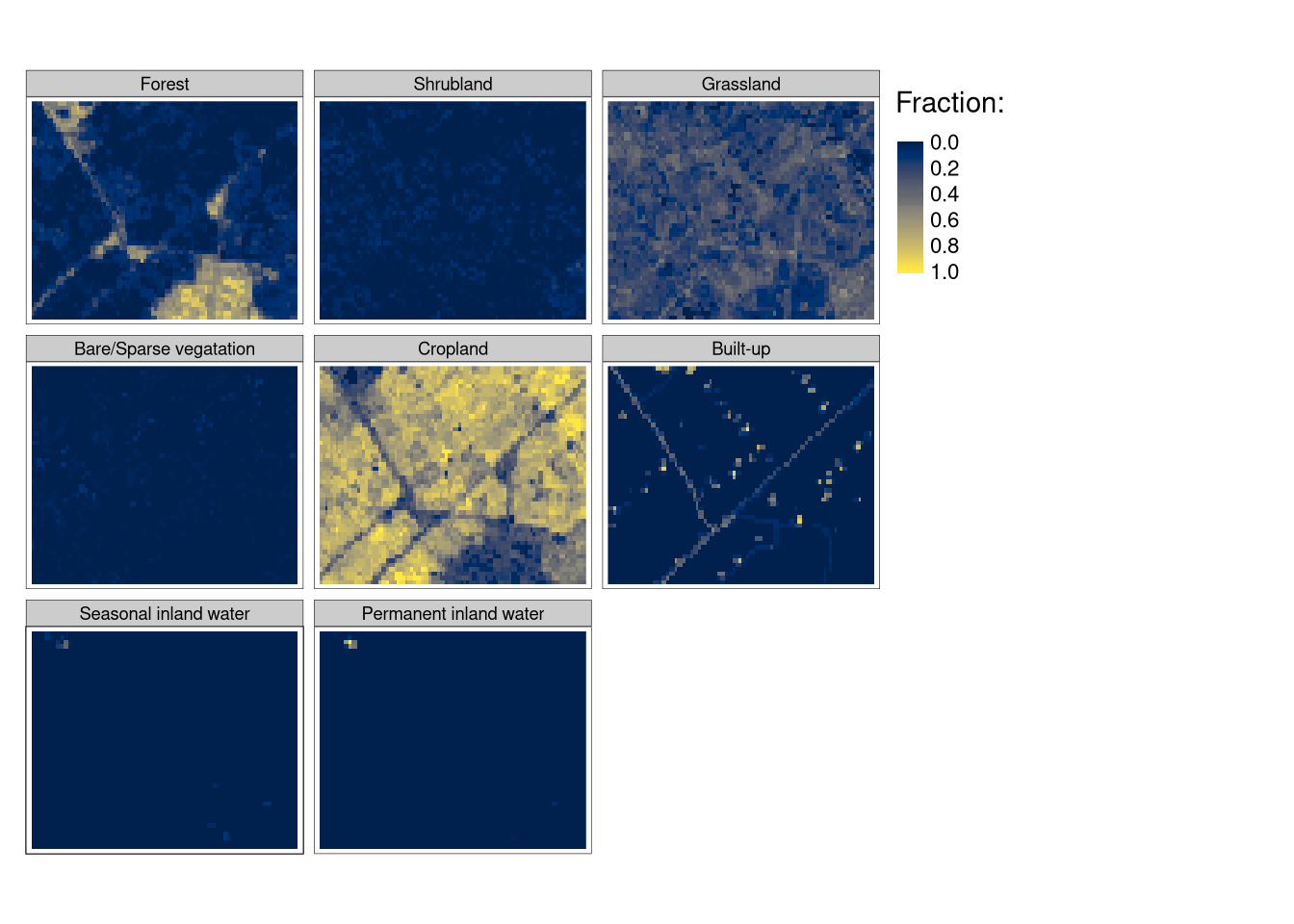
This blog post presents a short example of using spatial raster data with compositional information (histograms). For the study site located in the eastern Netherlands, we downloaded fractions of a pixel’s area covered by different land cover classes (source: Copernicus Global Land Service: 2019 Land Cover 100m-resolution data). Our goal is to create superpixels with similar fractions of land cover classes (Figure 1).
Let’s start by attaching the packages and reading the input data:
The input data, flc, is a raster of 507 by 1105 cells and eight layers (fractions of different land cover classes). We will resample our raster into a projected CRS and, for a simplicity case and to see our results easier, we will crop it to a 50 by 100 cells area:
flc1 = project(flc, "EPSG:3035", method = "near")
flc1 = flc[101:150, 1:100, drop = FALSE]
The flc1 object represents an area mostly covered by croplands, with some forests in its south-eastern parts, and smaller fractions of grasslands and built-up classes:
tm_shape(flc1) +
tm_raster(style = "cont", palette = "cividis", title = "Fraction:") 
Now, we are able to create supercells using the supercells package and its supercells() function.3 This function is very flexible and its results can be much customized.4 Here, we will just use its basic arguments:
x: our input raster with one or more layers;flc1in our casestep: our \(S\) interval between initial cluster centers; here we use the value of12(cells). Decreasing this value with give us more supercells, and increasing it results in fewer supercellscompactness: \(m\), the compactness parameter; here we use the value of0.1– the lower the value, the more impact the value distance has on the resultdist_fun: distance function used; here we use the Jensen-Shannon distance ("jensen-shannon"), which is suitable for measuring the dissimilarity between histograms
flc_sc = supercells(x = flc1,
                    step = 12, compactness = 0.1,
                    dist_fun = "jensen-shannon")
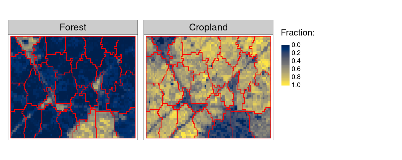
The flc_sc result is an sf (spatial vector) object with 28 polygons. We can visualize them on top of the two most prominent land cover classes for this area, forest and cropland (Figure 2):
tm_shape(flc1[[c(1, 5)]]) +
  tm_raster(style = "cont", palette = "cividis", title = "Fraction:") +
  tm_shape(flc_sc) +
  tm_borders(col = "red")
This visual inspection allows us to see that supercells serve their purpose: they delineate areas with homogeneous arrangements of fractional land cover values. Areas with dominating fractions of forests are encapsulated in different polygons compared to there with dominating fractions of croplands, or some mixes of land cover classes. At the same time, some supercells are more homogeneous than others. This is due to: (a) the set \(S\) interval value (a lower value would result in a large number of more homogeneous supercells), and (b) the fact that supercells are not designed especially for roads (or other linear features) detection.
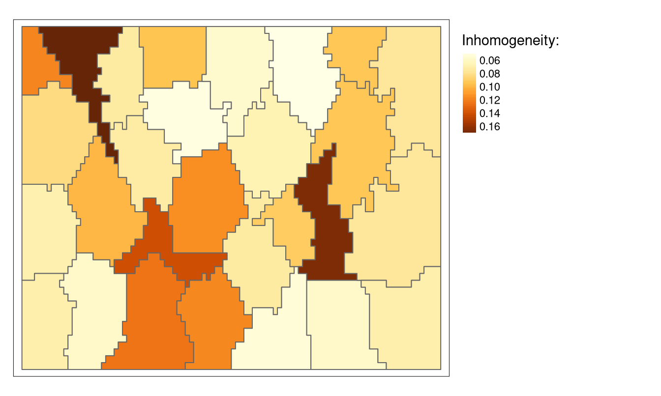
The quality of our result can also be determined numerically: we can calculate “inhomogeneity” of our supercells. The inhomogeneity metric represents an average distance between cells belonging to the same supercell. This value is small when all cells have similar values (land cover classes’ fractions, in our case), and large when cells’ values are very different.
Inhomogeneity can be calculated using the regional package’s function reg_inhomogeneity(). We just need to provide our “regions” (supercells), raster with values, and a distance function. Comparing values of many cells may take a lot of time; thus, usually, it is more efficient to use some subset of them for this comparison. We can specify the subset size with sample_size.
vars = c("Forest", "Shrubland", "Grassland", "Bare.Sparse.vegatation",
         "Cropland", "Built.up", "Seasonal.inland.water", "Permanent.inland.water")
flc_sc$inh = reg_inhomogeneity(flc_sc[vars], flc1,
                                dist_fun = "jensen-shannon", sample_size = 100)
The resulting inhomogeneity values can also be visualized, signaling the most and the least consistent supercells (Figure 3):
tm_shape(flc_sc) +
  tm_polygons("inh", title = "Inhomogeneity:", style = "cont") +
  tm_layout(legend.outside = TRUE)
Additionally, we can calculate an area-weighted inhomogeneity as a general metric of all the supercells:
flc_sc$area_km2 = as.numeric(st_area(flc_sc)) / 1000000
weighted.mean(flc_sc$inh, flc_sc$area_km2)
[1] 0.08516878Finally, you may notice that several adjacent supercells are very similar, and thus should be merged. Several approaches to merging supercells into larger segments/regions exist. I will discuss them in the next blog post.
Summary
We propose the SLIC algorithm extension to work with non-imagery data structures without data reduction and conversion to the false-color image. It allows for using a data distance measure most appropriate to a particular data structure and a custom function for averaging values of clusters centers. If you want to learn more about supercells, we encourage you to try a few entry points. One is the Nowosad and Stepinski (2022) article that explains the whole idea in more detail and compares our extension and original SLIC algorithms on three examples of non-imagery data. Code related to these examples is available at https://github.com/Nowosad/supercells-examples. You can also see slides from a talk entitled “A method for universal superpixels-based regionalization” that I gave during the FOSS4G 2022 conference at https://jakubnowosad.com/foss4g-2022/. Finally, the package has extensive documentation, including several vignettes, that can be found at https://jakubnowosad.com/supercells/.
References
Footnotes
On a side note: homogeneity does not always imply simplicity.↩︎
Let me know (email/twitter) if you have any examples of such data!↩︎
Supercells!↩︎
Read the “The supercells() function” vignette for more details.↩︎
Reuse
Citation
@online{nowosad2023,
  author = {Nowosad, Jakub},
  title = {Supercells: Universal Superpixels Algorithm for Applications
    to Geospatial Data},
  date = {2023-04-30},
  url = {https://jakubnowosad.com/posts/2023-04-30-supercells-bp1/},
  langid = {en}
}
