Extracting information about spatial patterns from spatial signatures

The spatial signatures of categorical rasters are a set of numbers that describe the spatial patterns of the provided variables. Next, they allow for further operations such as searching, comparing, or clustering. Less known is that they can also be used to extract information about the composition and configuration of spatial patterns. This blog post shows how to do it using the motif R package.

Spatial data

To reproduce the calculations in the following post, you need to download all of the relevant datasets using the code below:

library(osfr)
dir.create("data")
osf_retrieve_node("xykzv") |>
        osf_ls_files(n_max = Inf) |>
        osf_download(path = "data",
                     conflicts = "skip")

You should also attach the following packages:

library(sf)
library(terra)
library(motif)
library(dplyr)
library(readr)
library(cluster)
library(ggplot2)

Land cover in Africa

The data/land_cover.tif contains land cover data for Africa. It is a categorical raster of the 300-meter resolution that can be read into R using the rast() function.

lc = rast("data/land_cover.tif")

Additionally, the data/lc_palette.csv file contains information about the labels and colors of each land cover category.

lc_palette_df = read.csv("data/lc_palette.csv")

We will use this file to integrate labels and colors into the raster object:

levels(lc) = lc_palette_df[c("value", "label")]
coltab(lc) = lc_palette_df[c("value", "color")]
plot(lc)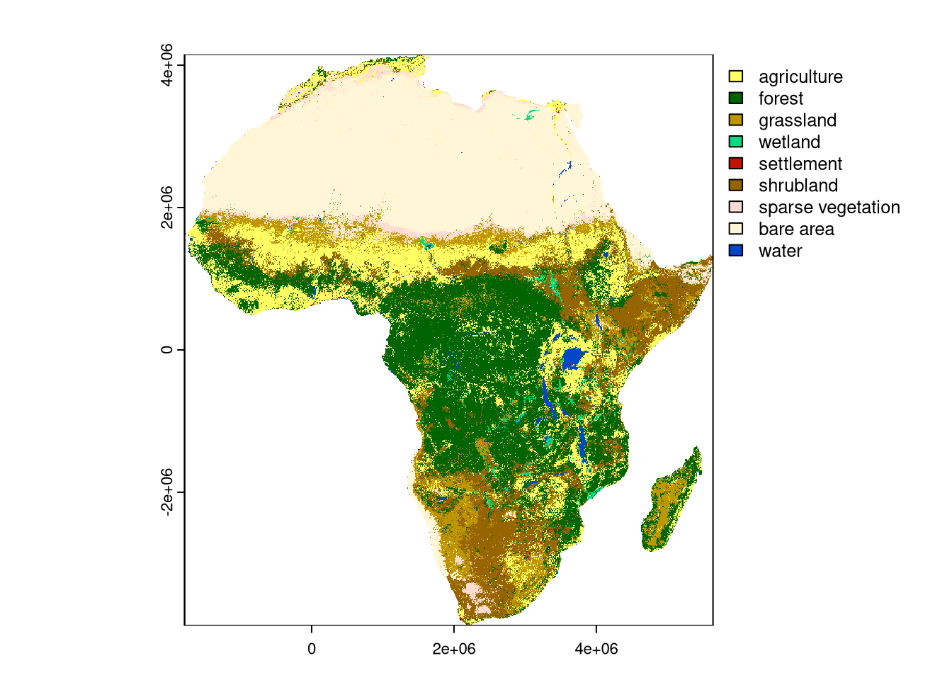

Extracting information from spatial signatures

As already shown in the previous blog posts about motif, the lsp_signature() function can be used to extract spatial signatures from a categorical raster object that can be used to describe spatial patterns of land cover. The most fundamental signature is co-occurrence matrix (coma), which is a matrix of co-occurrence frequencies of each pair of land cover categories. The lsp_signature() function can be used to extract the coma signature in 300 by 300 cells non-overlapping windows (i.e., 90 by 90 km) as follows:

lc_coma = lsp_signature(lc, type = "coma", window = 300)

The output is a data frame with 3,843 rows and 3 columns. The most important one is the signature column, which contains coma signatures in each window.

The co-occurrence matrix can be thought of as a compression of information about the composition and configuration of land cover categories in a given window. However, as it consists of many numbers (here, 81), it is not easy to directly analyze, visualize, or interpret. Gladly, we can further extract information from this signature using metrics from the information theory, such as marginal entropy and relative mutual information (for more details, see Nowosad and Stepinski (2019) and the “Information theory provides a consistent framework for the analysis of spatial patterns” blog post).

The it_metric() function from the comat package can be used to calculate these metrics for each coma signature. Here, we calculate marginal entropy ("ent") and relative mutual information ("relmutinf"), and add them to the lc_coma data frame.

lc_coma$ent = vapply(lc_coma$signature, comat::it_metric,
       FUN.VALUE = numeric(1), metric = "ent")
lc_coma$relmutinf = vapply(lc_coma$signature, comat::it_metric,
       FUN.VALUE = numeric(1), metric = "relmutinf")

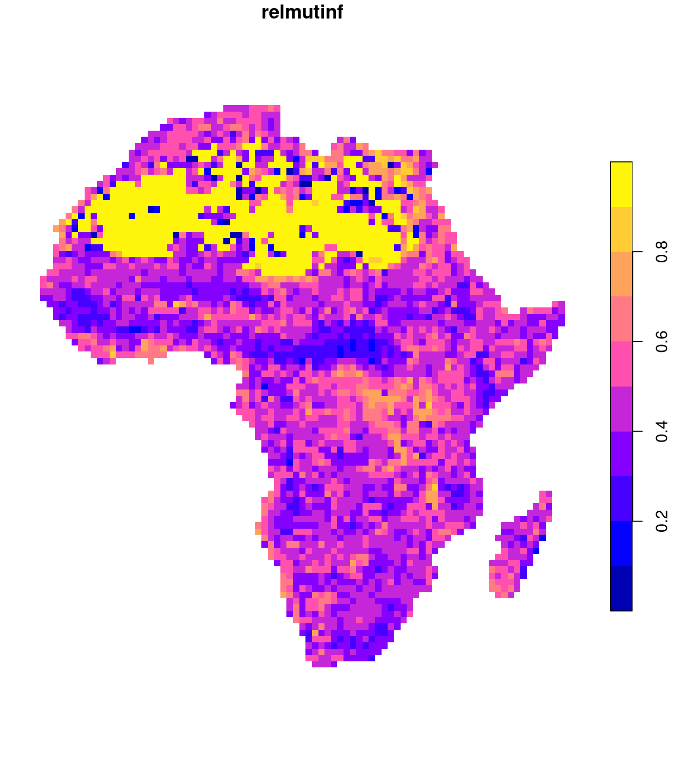
In short, the marginal entropy is a measure of diversity (thematic complexity, composition) of spatial categories — the larger the entropy, the more diverse the categories in the window. The relative mutual information is a measure of spatial autocorrelation (configuration) of spatial categories – the larger the relative mutual information, the more autocorrelated the categories in the window are.

Importantly, both metrics are uncorrelated, which means that they describe different aspects of spatial patterns of land cover:

plot(lc_coma$ent, lc_coma$relmutinf)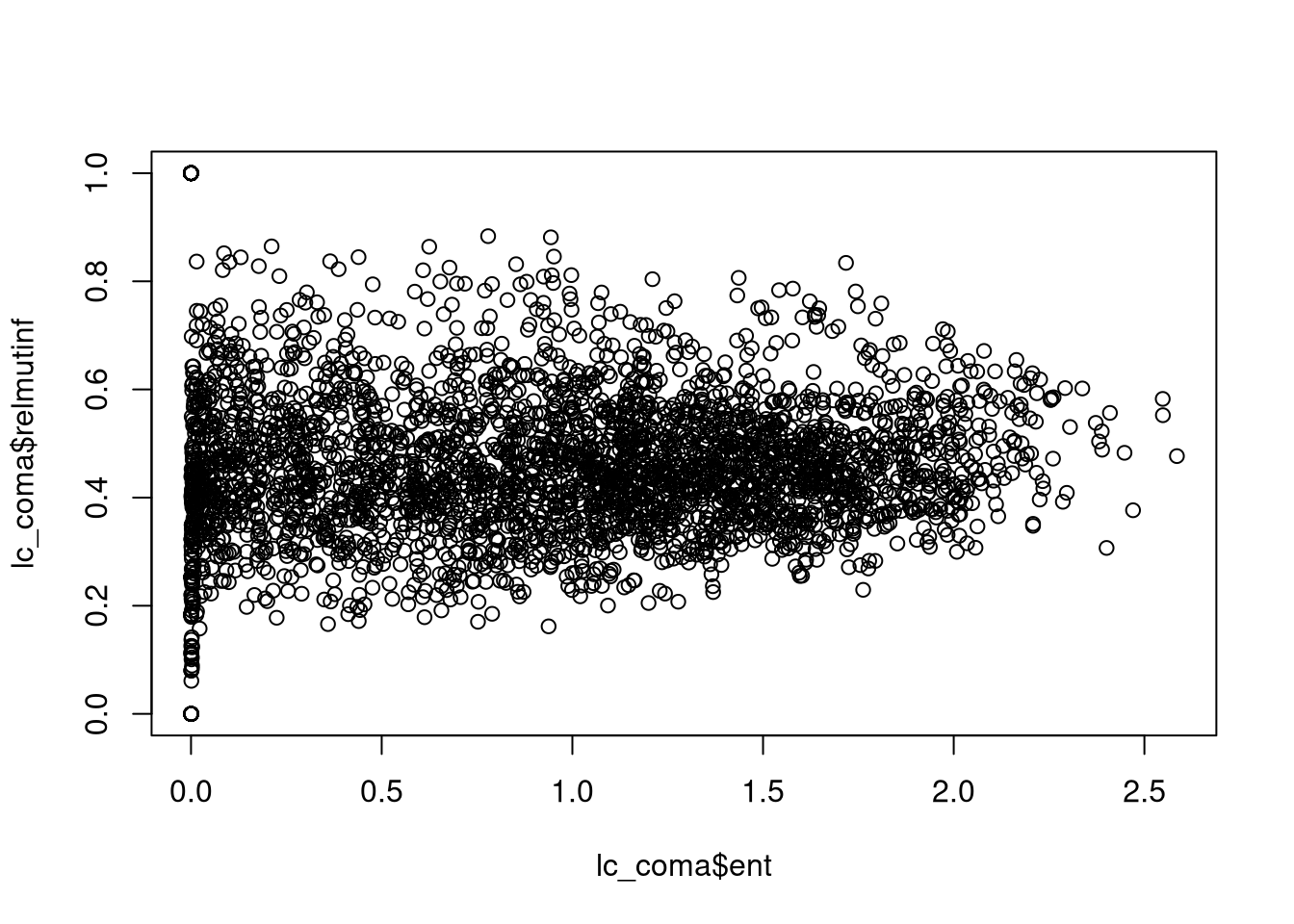

Visualizing spatial patterns’ metrics

We can visualize the spatial distribution of these metrics’ values by removing the signature column and converting the lc_coma object to an sf class:

lc_coma$signature = NULL
lc_coma_sf = lsp_add_sf(lc_coma)
plot(lc_coma_sf["ent"], border = NA)
plot(lc_coma_sf["relmutinf"], border = NA)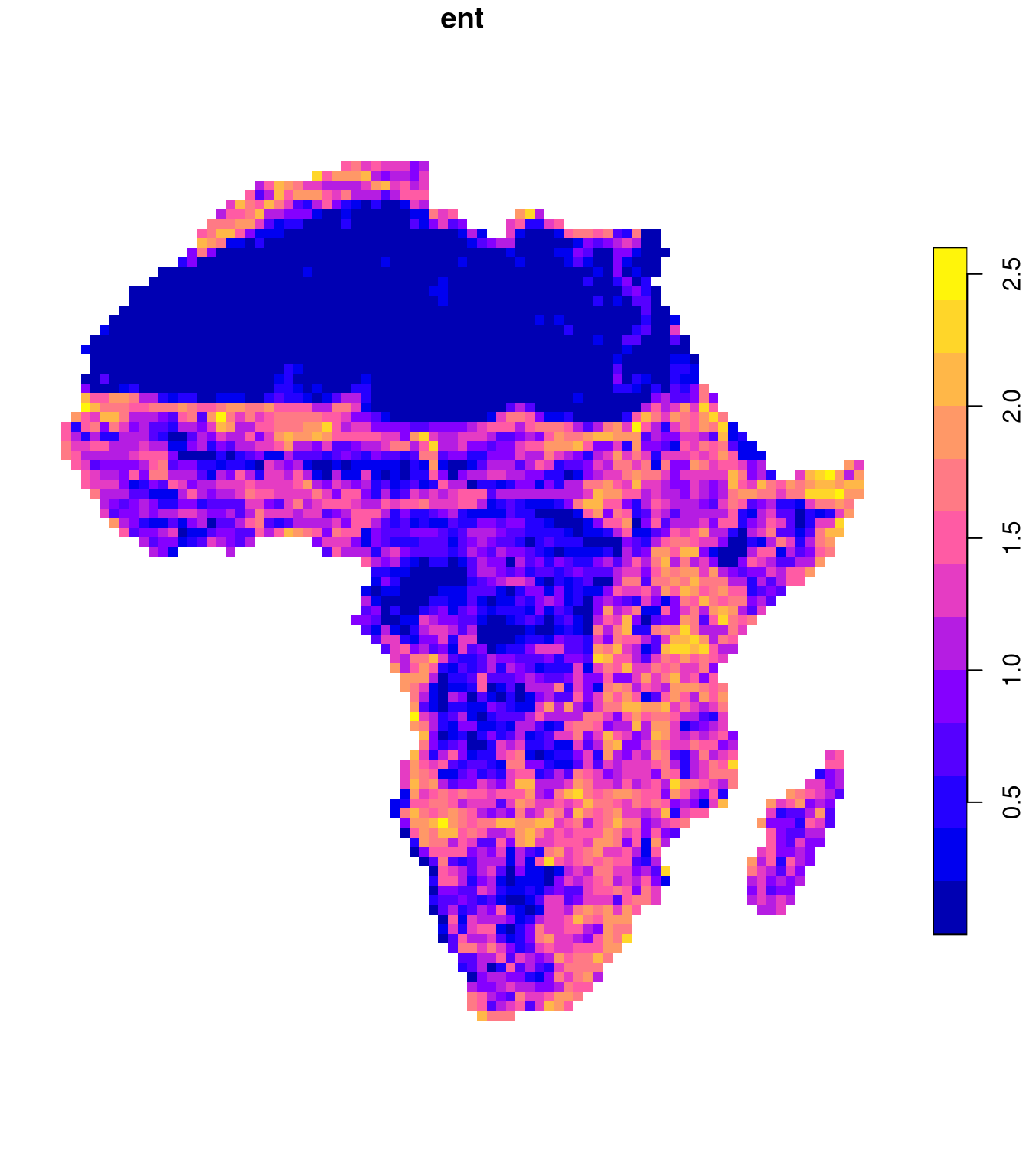

Representative examples

We are also able to look at some examples of areas with representative values of these metrics. For that purpose, we use the pam() method (Partitioning Around Medoids) to cluster the lc_coma data frame into six groups based on the scaled values of ent and relmutinf.

pam = pam(scale(lc_coma[, c("ent", "relmutinf")]), 6)

We can see all of the groups on the map by adding a new column with cluster labels to the lc_coma_sf object and plotting it:

lc_coma_sf$cluster = pam$clustering
plot(lc_coma_sf["cluster"], border = NA, pal = palette.colors(6))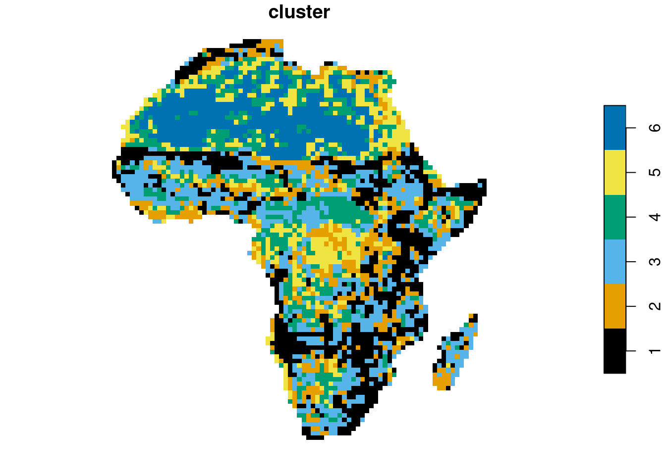

Then, we can select one representative from each cluster in a loop using the crop() function and visualize it using plot().

lc_coma_sf_subset = lc_coma_sf[pam$id.med, ]
for (i in seq_len(nrow(lc_coma_sf_subset))){
  ent_sel = round(lc_coma_sf_subset[i, "ent", drop = TRUE], 2)
  relmutinf_sel = round(lc_coma_sf_subset[i, "relmutinf", drop = TRUE], 2)
  plot(crop(lc, lc_coma_sf_subset[i, ]), 
       main = paste0(i, " ent: ",  ent_sel, " relmutinf: ", relmutinf_sel))
}

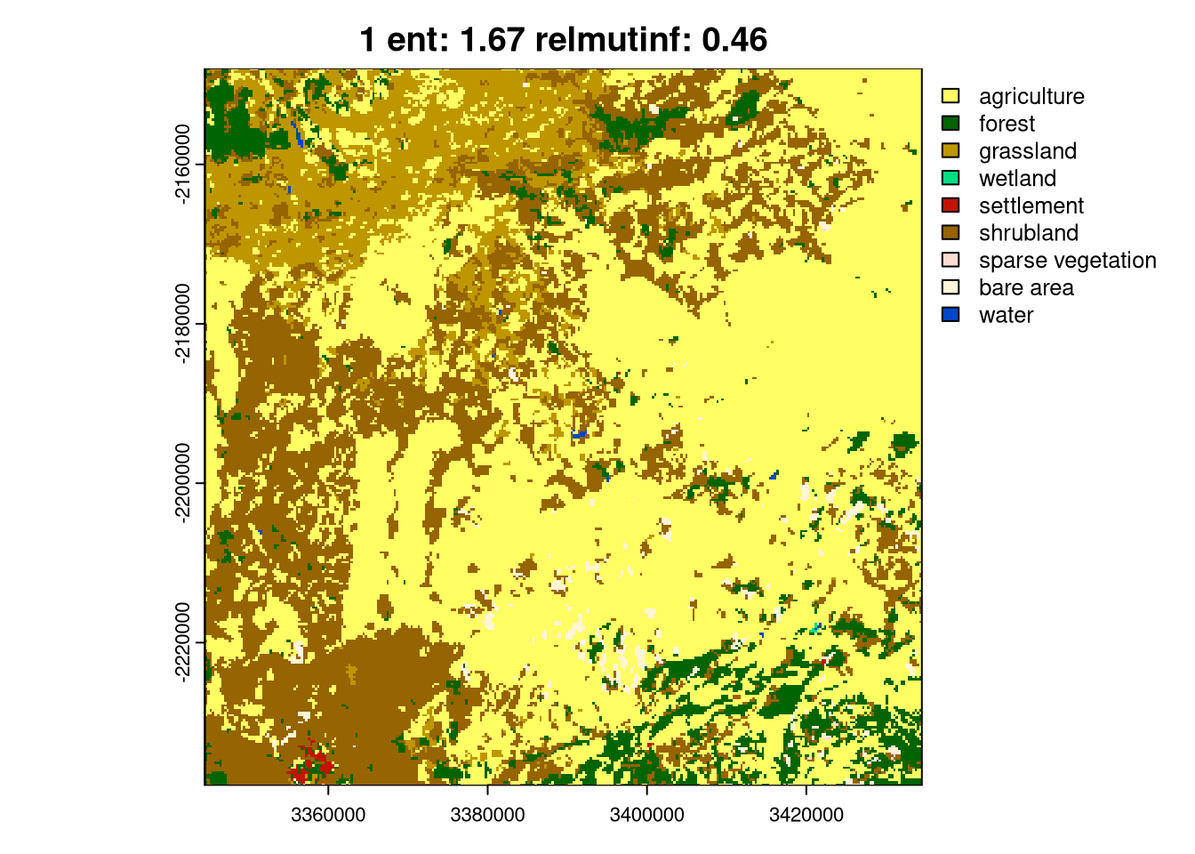
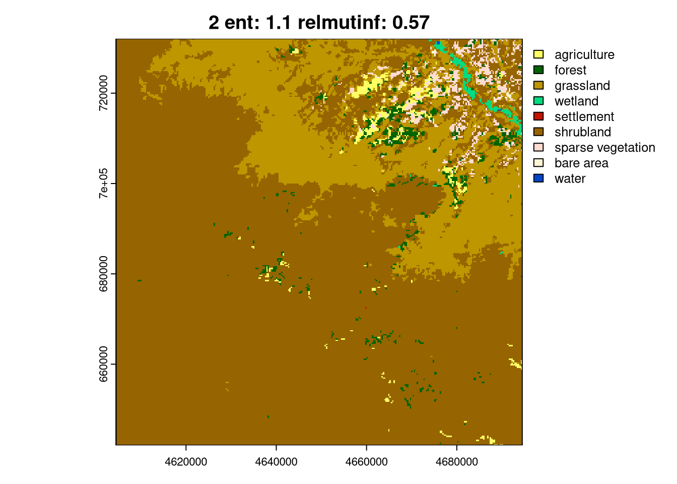
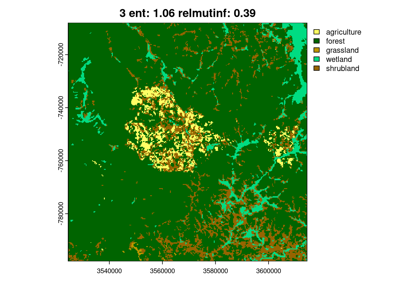
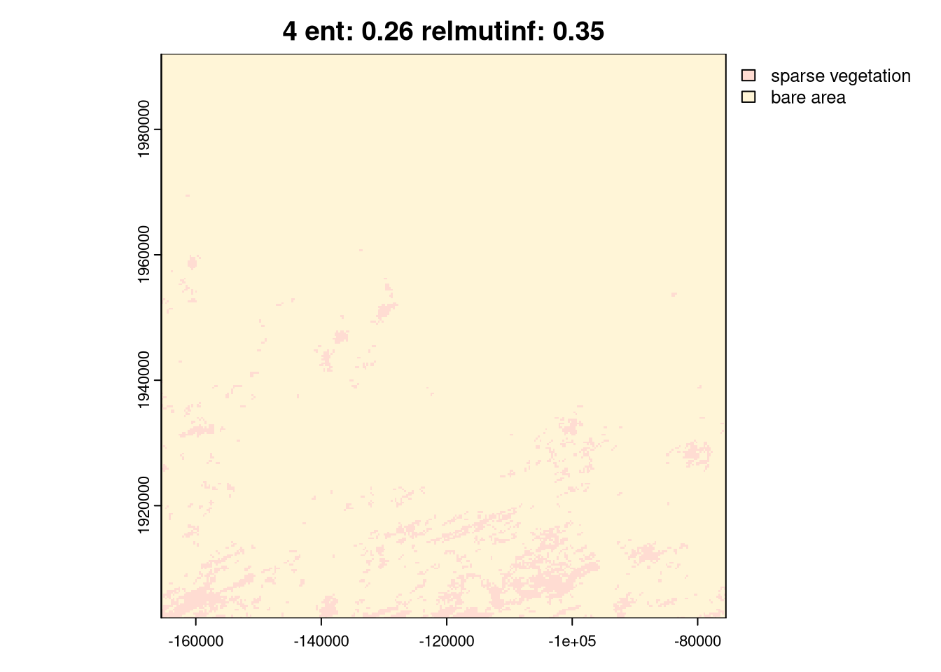
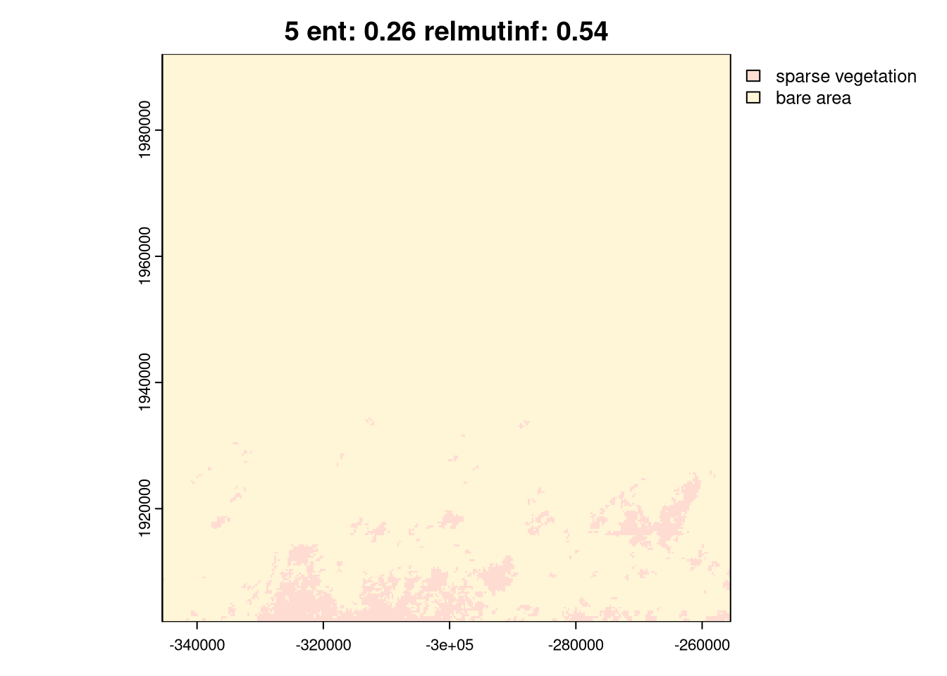
As you can see above, the ent and relating metrics can be used to describe various spatial patterns of land cover. The last group, 6, is the simplest one with just one land cover category. Next, groups 4 and 5 represent areas with a low diversity of land cover categories but with different spatial autocorrelation: Group 4 has lower spatial autocorrelation (is more fragmented), while group 5 has higher spatial autocorrelation (is less fragmented). Groups 2 and 3 are areas with medium diversity of land cover categories, but with different spatial autocorrelation: group 2 has higher spatial autocorrelation, while group 3 has lower spatial autocorrelation. Finally, group 1 is an area with a high diversity of land cover categories and a medium spatial autocorrelation.

Additional possibilities

Importantly, these metrics do not provide any information about the actual land cover categories. Thus, to look at the results in more depth, we can add information about land cover shares in each window to the lc_coma_sf data frame and use it in further analysis.

Here, we can use the "composition" type of signature to extract information about land cover shares in each window, restructure it from a list column to a set of columns, and add it to the lc_coma_sf data frame.

lc_composition = lsp_signature(lc, type = "composition", window = 300)
lc_composition = lsp_restructure(lc_composition)
lc_coma_sf = left_join(lc_coma_sf, lc_composition)

Now, you are able to subset your data frame based on the land cover shares and analyze the spatial patterns for various types of areas. You can also repeat the above calculations for two time periods or two areas and compare the results.

Summary

This blog post shows how to extract information about the composition and configuration of spatial patterns, visualize it on a map, and look at representative examples. For more details about the information theory-based metrics, see the “Information theory provides a consistent framework for the analysis of spatial patterns” blog post. To learn more about the motif package, see the other blog posts in the “motif” category.

References

Nowosad, Jakub, and Tomasz F. Stepinski. 2019. “Information Theory as a Consistent Framework for Quantification and Classification of Landscape Patterns.” Landscape Ecology 34 (9): 2091–101. https://doi.org/10.1007/s10980-019-00830-x.