clc_diff = clc2018_tartu != clc2000_tartu
plot(clc_diff)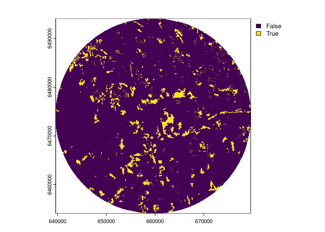
November 3, 2024
This is the fourth part of a blog post series on comparing spatial patterns in raster data. More information about the whole series can be found in part one.
This blog post focuses on the comparison of spatial patterns in categorical raster data for overlapping regions. In other words, here we have two rasters with the same number of rows and columns, and we want to compare their spatial patterns.
For this blog post, we use two categorical raster datasets: the CORINE Land Cover (CLC) datasets for Tartu (Estonia) for the years 2000 and 2018.
library(terra)
clc2000_tartu = rast("https://github.com/Nowosad/comparing-spatial-patterns-2024/raw/refs/heads/main/data/clc2000_tartu.tif")
clc2018_tartu = rast("https://github.com/Nowosad/comparing-spatial-patterns-2024/raw/refs/heads/main/data/clc2018_tartu.tif")
plot(clc2000_tartu, main = "Tartu (2000)")
plot(clc2018_tartu, main = "Tartu (2018)")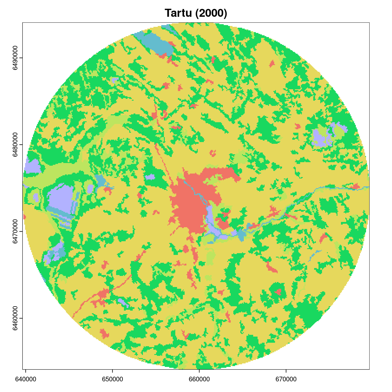
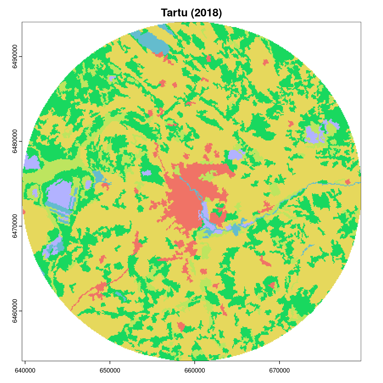
In short, the red areas in the rasters represent urban areas, the green areas represent forests, the blue areas represent water bodies, and the yellow areas represent agricultural land.
The simplest way to compare two categorical rasters is to create a binary raster that indicates whether the values of the two rasters are the same or different. Here, the output highlights the areas where the values of the two rasters differ (yellow) and where they are the same (purple).
To get a more detailed comparison, we can calculate the confusion matrix (also known as, e.g., contingency table) of the two rasters. It shows the number of pixels that have the same value in both rasters (diagonal) and the number of pixels with different values (off-diagonal).
        1     2     3     4     6     7
  1  4821   357     2    10     0     0
  2  1342 67915   684   389     0     0
  3    59   415 33670  2896     9    22
  4   122   638  1435  7040   229    24
  6     0     3    13    20  2177    37
  7     0     0     0     0     3  1995
For example, the table shows that there are 4821 pixels with the value 1 in both rasters, and 357 pixels with the value 2 in the first raster and the value 1 in the second raster.
Confusion matrices is also a building block for many other statistics, including accuracy, that can be calculated to compare the two sets of categorical data.
A binary difference raster can be also used to calculate the proportion of changed pixels by dividing the number of changed pixels by the total number of non-NA pixels.
[1] 0.06894013This outcome shows that about 0.07 of the pixels have changed between the two rasters.
The overall comparison of the two rasters can be done by calculating the difference between the frequencies of the values of the two rasters (Pontius 2002).
clc2000_tartu_freq = freq(clc2000_tartu)
clc2018_tartu_freq = freq(clc2018_tartu)
freq = merge(clc2000_tartu_freq, clc2018_tartu_freq, by = "value", all = TRUE)
freq$diff = abs(freq$count.x - freq$count.y)
sum_diff = sum(freq$diff)
na_pixels = freq(clc_diff, value = NA)$count
total_pixels = ncell(clc_diff) - na_pixels
1 - sum_diff / total_pixels
[1] 0.9640774The overall comparison tells what is the percentage of pixels that have the same class in both rasters (however, it does not consider if the pixels are in the same location).
More statistics of the differences between the values of the two rasters can be calculated using the diffeR package (Pontius Jr. and Santacruz 2023). These statistics are based on the confusion matrix and include the overall allocation disagreement, overall difference, overall exchange disagreement, overall quantity disagreement, and overall shift disagreement.1
  overallAllocD overallDiff overallExchangeD overallQtyD overallShiftD
1 6440 8709 5280 2269 1160To include the spatial context in the comparison, we can calculate the difference between a focal measure of two rasters. An example of such a measure is the relative mutual information (relmutinf) metric, which quantifies the clumpiness of the landscape – the larger the value, the more clumped the landscape is [^See a blog post about this metric].
The below code chunk uses the landscapemetrics package (Hesselbarth et al. 2019) to specify a moving window of 5 by 5 and calculate the relmutinf metric for the two rasters. Next, it calculates the absolute difference between the two rasters and plots the result.
library(landscapemetrics)
window = matrix(1, nrow = 5, ncol = 5)
clc2000_tartu_relmutinf_mw = window_lsm(clc2000_tartu, window = window,
                                        what = "lsm_l_relmutinf")
clc2018_tartu_relmutinf_mw = window_lsm(clc2018_tartu, window = window,
                                        what = "lsm_l_relmutinf")
clc2018_tartu_relmutinf_diff = abs(clc2018_tartu_relmutinf_mw[[1]][[1]] -
                                   clc2000_tartu_relmutinf_mw[[1]][[1]])
plot(clc2018_tartu_relmutinf_diff)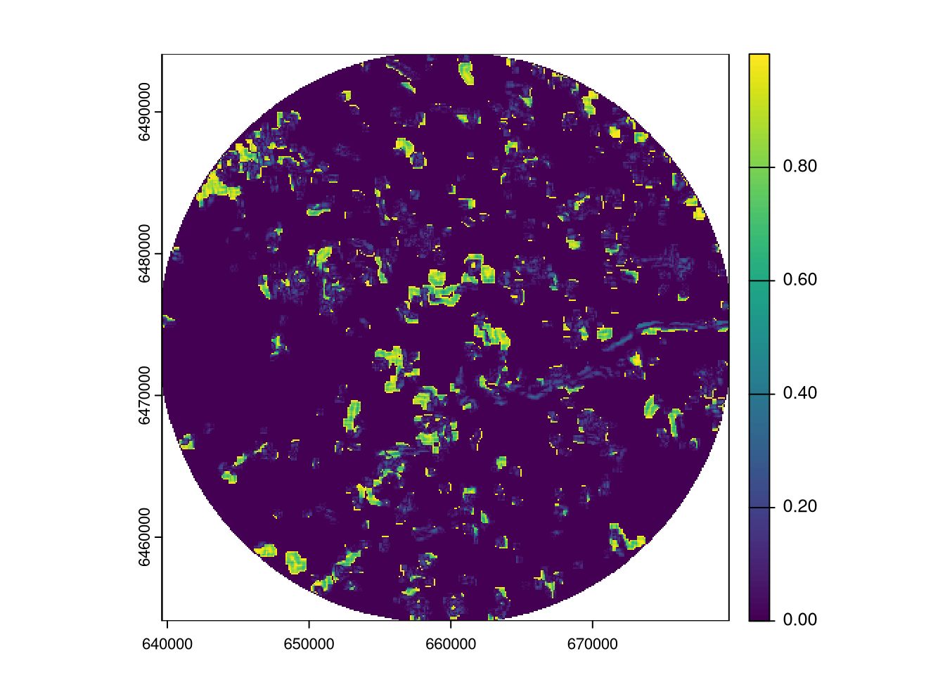
The largest values in the output indicate the areas where the clumpiness of the landscape has changed the most between the two rasters.
Alternatively, if we calculate the regular difference, the output will show the areas where the clumpiness of the landscape has increased (positive values) and decreased (negative values).
plot_div = function(r, ...){
  r_range = range(values(r), na.rm = TRUE, finite = TRUE)
  max_abs = max(abs(r_range))
  new_range = c(-max_abs, max_abs)
  plot(r, col = hcl.colors(100, palette = "prgn"), range = new_range, ...)
}
clc2018_tartu_relmutinf_diff2 = clc2018_tartu_relmutinf_mw[[1]][[1]] -
                                clc2000_tartu_relmutinf_mw[[1]][[1]]
plot_div(clc2018_tartu_relmutinf_diff2)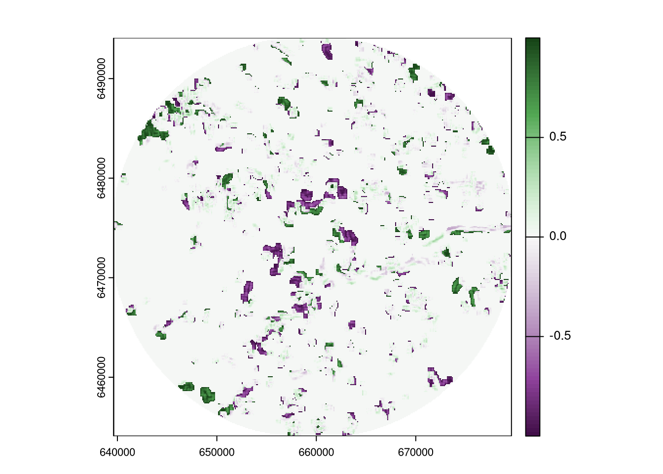
The moving window approach is also used in the raster.change() function from the spatialEco package (Evans and Murphy 2023). Its first two arguments are the two rasters to compare, the s argument specifies the size of the moving window, and the stat argument specifies the statistic to calculate. For example, stat = "cross-entropy" calculates the cross-entropy loss function, where the larger the value, the more different the two rasters are.
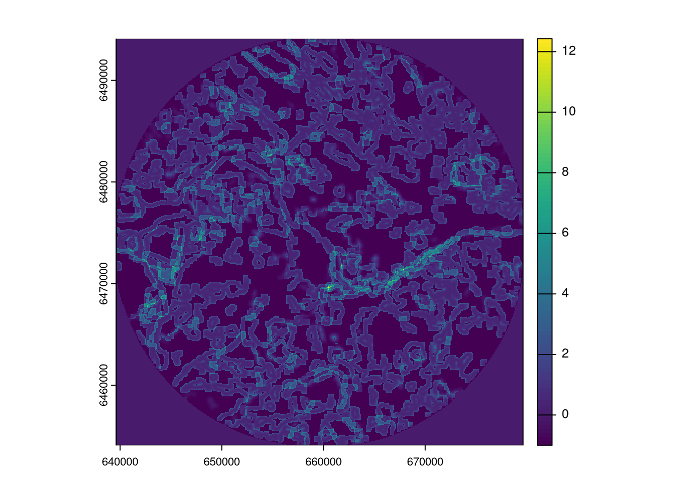
Note that the above calculation may take a few minutes to complete.
Various statistics from categorical data can be calculated at multiple scales with the waywiser package (Mahoney 2023). Here, the ww_multi_scale() function calculates the accuracy of the two rasters at different scales from 500 to 3000 meters (map units).
# A tibble: 6 × 6
  .metric  .estimator .estimate .grid_args       .grid            .notes
  <chr>    <chr>          <dbl> <list>           <list>           <list>
1 accuracy multiclass     0.781 <tibble [1 × 1]> <sf [6,400 × 5]> <tibble>
2 accuracy multiclass     0.607 <tibble [1 × 1]> <sf [1,600 × 5]> <tibble>
3 accuracy multiclass     0.453 <tibble [1 × 1]> <sf [729 × 5]>   <tibble>
4 accuracy multiclass     0.358 <tibble [1 × 1]> <sf [400 × 5]>   <tibble>
5 accuracy multiclass     0.246 <tibble [1 × 1]> <sf [256 × 5]>   <tibble>
6 accuracy multiclass     0.270 <tibble [1 × 1]> <sf [196 × 5]>   <tibble>
The output shows the accuracy of the two rasters at each scale: the largest value is at the scale of 500 meters, and the smallest value is at the scale of 3000 meters. It shows that with the increase of the scale, the agreement between the two rasters decreases – both rasters are similar at the local scale, but they differ at the regional one.
The sabre package (Nowosad and Stepinski 2018) provides a function to calculate a few measures of spatial association between two categorical maps.2
The SABRE results:

 V-measure: 0.77
 Homogeneity: 0.78
 Completeness: 0.76

 The spatial objects can be retrieved with:
 $map1 - the first map
 $map2 - the second map
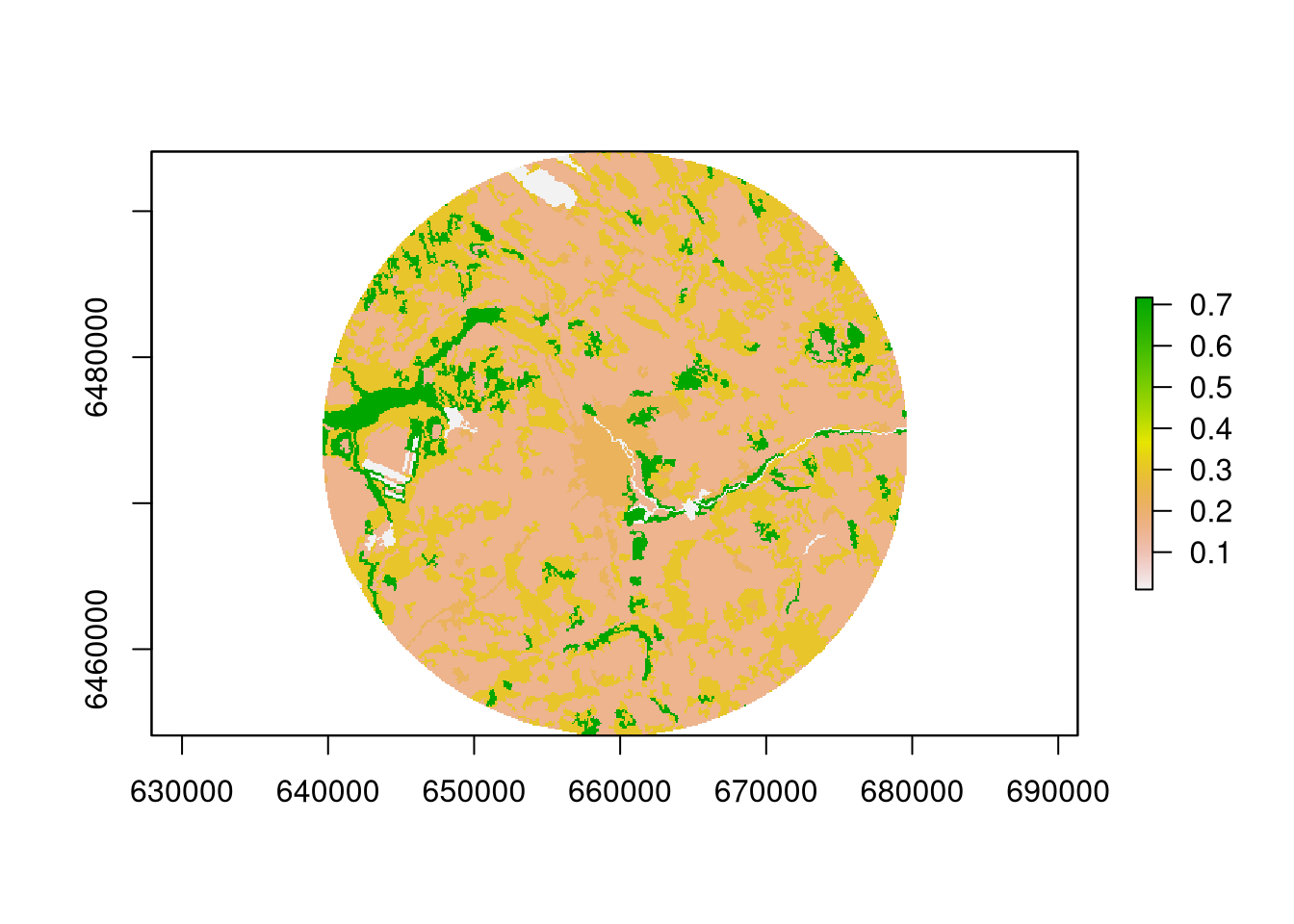
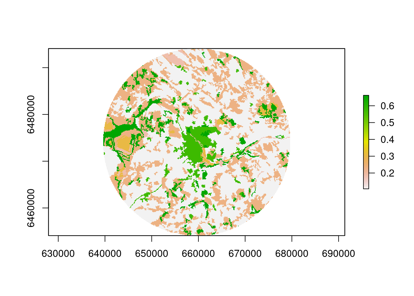
Its output returns three values: the homogeneity, the completeness, and the V-measure. The homogeneity measures how well regions from the first map fit inside of regions from the second map, the completeness measures how well regions from the second map fit inside of regions from the first map, and the V-measure is the weighted harmonic mean of homogeneity and completeness. All of them range from 0 to 1, where larger values indicate better spatial agreement.
Additionally, the output contains two sets of maps of regions’ inhomogeneities (rih): the first set shows how the regions from the first map are inhomogenous in regard to the regions from the second map, and the second set shows how the regions from the second map are inhomogenous in regard to the regions from the first map.
@online{nowosad2024,
  author = {Nowosad, Jakub},
  title = {Comparison of Spatial Patterns in Categorical Raster Data for
    Overlapping Regions Using {R}},
  date = {2024-11-03},
  url = {https://jakubnowosad.com/posts/2024-11-03-spatcomp-bp4/},
  langid = {en}
}