sabre: Spatial Association Between REgionalizations - raster data
Jakub Nowosad
2024-12-14
Source:vignettes/sabre2.Rmd
sabre2.RmdThe sabre (Spatial
Association Between
REgionalizations) is an R package for calculating a
degree of spatial association between regionalizations or categorical
maps. This package offers support for sf,
RasterLayer, SpatRaster, and
stars spatial objects, and the following methods:
- the V-measure method (Nowosad and Stepinski, 2018)
- the MapCurve method (Hargrove et al., 2006)
Basic example - SABRE
Two simple regionalizations would be used to show the basic concept of sabre.
library(sabre)
#> Warning: multiple methods tables found for 'area'
#> Warning: multiple methods tables found for 'gridDistance'
library(raster)
data("partitions1")
data("partitions2")
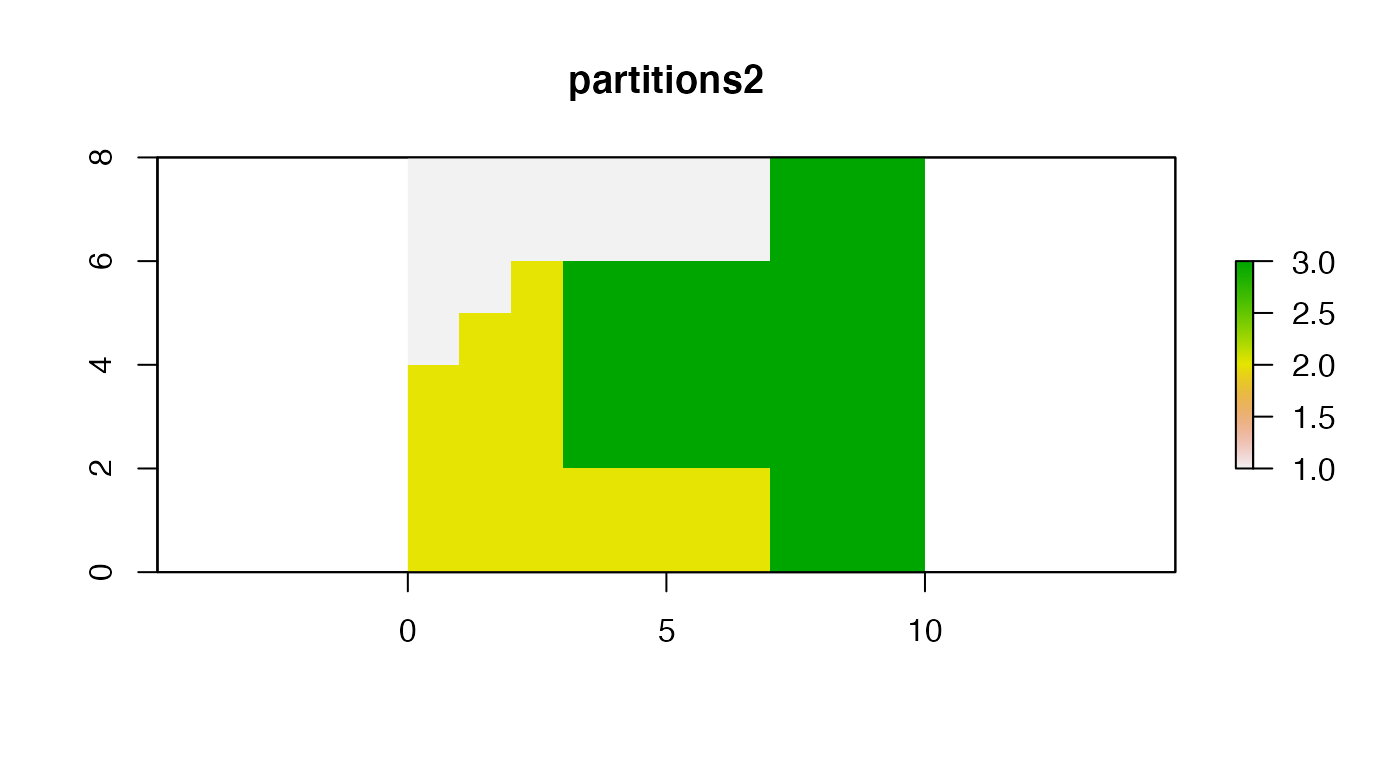
The first map, partitions1, has four regions (“r1”,
“r2”, “r3”, “r4”) of the same size and shape. The second one,
partitions2, contains three irregular regions where “z1” is
the smallest and “z3” being the largest. Our goal is to compare these
two regionalizations and calculate a degree of spatial association
between them.


It can be done with vmeasure_calc(), which calculates
“V-measure”, “Homogeneity”, and “Completeness” and returns two
preprocessed input maps. For raster data, this function requires, at
least, two arguments:
-
x- anRasterLayer,SpatRaster, orstarsobject containing the first regionalization -
y- anRasterLayer,SpatRaster, orstarsobject containing the second regionalization
Importantly, both x and y must have the
same coordinate reference system.
There are also one additional argument - B. If
B > 1 then completeness is weighted more strongly than
homogeneity, and if B < 1 then homogeneity is weighted
more strongly than completeness. By default this value is 1.
partitions_vm = vmeasure_calc(x = partitions1, y = partitions2)
partitions_vm
#> The SABRE results:
#>
#>  V-measure: 0.36
#>  Homogeneity: 0.32
#>  Completeness: 0.42
#>
#>  The spatial objects can be retrieved with:
#>  $map1 - the first map
#>  $map2 - the second map
The result is a list with three metrics of spatial association -
V-measure, Homogeneity,
Completeness - and two RasterLayer objects
with preprocessed input maps - $map1 and
$map2. All of the above metrics are between 0 and 1, where
larger values are desired. V-measure is a measure of an
overall spatial correspondence between input maps.
Homogeneity shows an average homogeneity of the regions in
the second map with respect to the regions in the first map.
Completeness is a function of homogeneity of the regions in
the first map with respect to the regions in the second map. The spatial
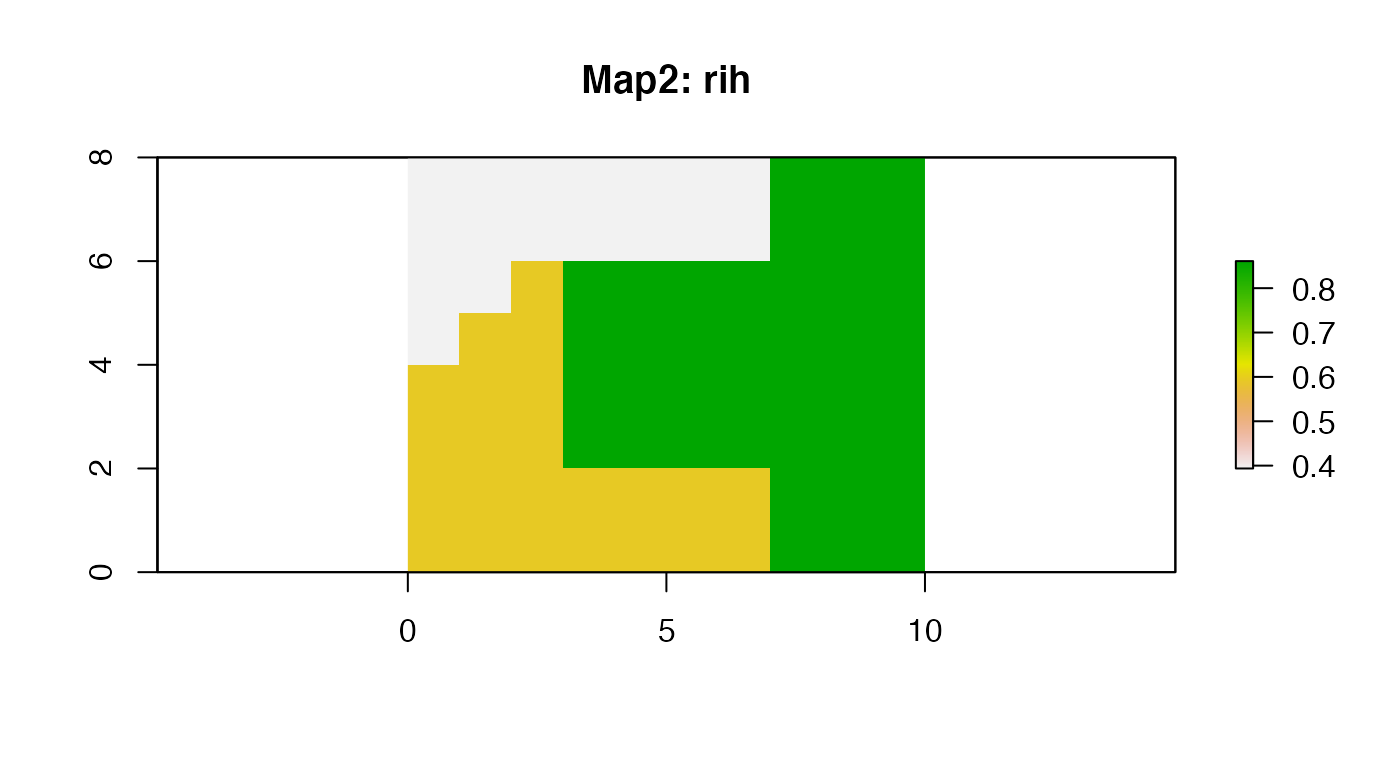
outputs, $map1 and $map2, have two layers. The
first one contains regions’ names and the second one (rih)
describes regions’ inhomogeneities.


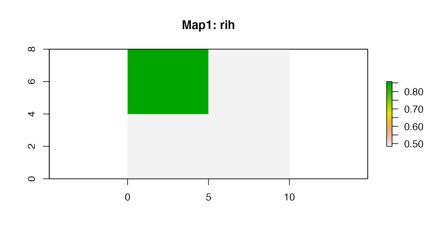
For example, “Map1” shows that three regions have the same inhomogeneity of 0.48. This is due a fact that all of these three have two regions from the second map. The upper left region has a larger inhomogeneity of 0.86 as its area “belongs” to three different regions in the second map. More information about this method and its applications can be found in Nowosad and Stepinski (2018).
Basic example - MapCurves
The sabre also allows for calculating a degree of
spatial association between regionalizations using the MapCurve method
(Hargrove et al., 2006). The mapcurves_calc() function also
requires two arguments, x and y. All of these
arguments are explained in the previous section.
partitions_mc = mapcurves_calc(x = partitions1, y = partitions2)
partitions_mc
#> The MapCurves results:
#>
#>  The goodness of fit: 0.61
#>  Reference map: x
#>
#>  The spatial objects can be retrieved with:
#>  $map1 - the first map
#>  $map2 - the second map
The mapcurves_calc() returns a list with a value of the
goodness of fit (GOF), the map used as a reference, and two
raster objects with preprocessed input maps -
$map1 and $map2. Read Hargrove et al. (2006)
to learn more about this method.
References
- Nowosad, Jakub, and Tomasz F. Stepinski. “Spatial association between regionalizations using the information-theoretical V-measure.” International Journal of Geographical Information Science (2018). https://doi.org/10.1080/13658816.2018.1511794
- Rosenberg, Andrew, and Julia Hirschberg. “V-measure: A conditional entropy-based external cluster evaluation measure.” Proceedings of the 2007 joint conference on empirical methods in natural language processing and computational natural language learning (EMNLP-CoNLL). 2007.
- Hargrove, William W., Forrest M. Hoffman, and Paul F. Hessburg. “Mapcurves: a quantitative method for comparing categorical maps.” Journal of Geographical Systems 8.2 (2006): 187.