Analysis of Spatial Patterns:
Current State and Future Challenges
2023-09-28
Hello, I am Jakub
Website: https://jakubnowosad.com/
- Computational geographer working at the intersection between geocomputation and the environmental sciences
- Assistant professor at the Adam Mickiewicz University, Poznan, Poland
- Main scientific interest: spatial pattern analysis, focusing on quantifying and understanding patterns in environmental data
- Co-author of a few books and textbooks on geocomputation and spatial analysis with R and Python, including “Geocomputation with R”
- Creator and contributor of various R packages for spatial data processing and visualization
- Educator, teaching courses on geocomputation, spatial analysis, programming, and data visualization
![]()
Acknowledgments
My family
Space Informatics Lab
![]()
The r-spatialecology organization
Many open-source contributors and inspirations
Spatial patterns
Discovering and describing patterns is a vital part of many spatial analysis However, spatial data is gathered in many ways and stored in forms, which requires different approaches to understanding spatial patterns
Spatial patterns of categorical rasters
Discovering and describing spatial patterns is an important part of many geographical studies, and spatial patterns are linked to natural and social processes.
Evaluation of the susceptibility of forest landscapes to agricultural expansion
Bourgoin et al., 2020, 10.1016/j.jag.2019.101958
Reinterpretation of histological images as categorized rasters and their use for disease classification (e.g., liver cancer)
Kendall et al., 2020, 10.1038/s41598-020-74691-9
Quantification of categorical spatial patterns
Spatial patterns can be quantified using landscape metrics (O’Neill et al. 1988; Turner and Gardner 1991; Li and Reynolds 1993; He et al. 2000; Jaeger 2000; Kot i in. 2006; McGarigal 2014).
Software such as FRAGSTATS, GuidosToolbox, or landscapemetrics has proven useful in many scientific studies (> 12,000 citations).
There is a relationship between an area’s pattern composition and configuration and ecosystem characteristics, such as vegetation diversity, animal distributions, and water quality within this area (Hunsaker i Levine, 1995; Fahrig i Nuttle, 2005; Klingbeil i Willig, 2009; Holzschuh et al., 2010; Fahrig et al., 2011; Carrara et al., 2015; Arroyo-Rodŕıguez et al. 2016; Duflot et al., 2017, many others..)
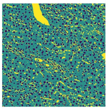
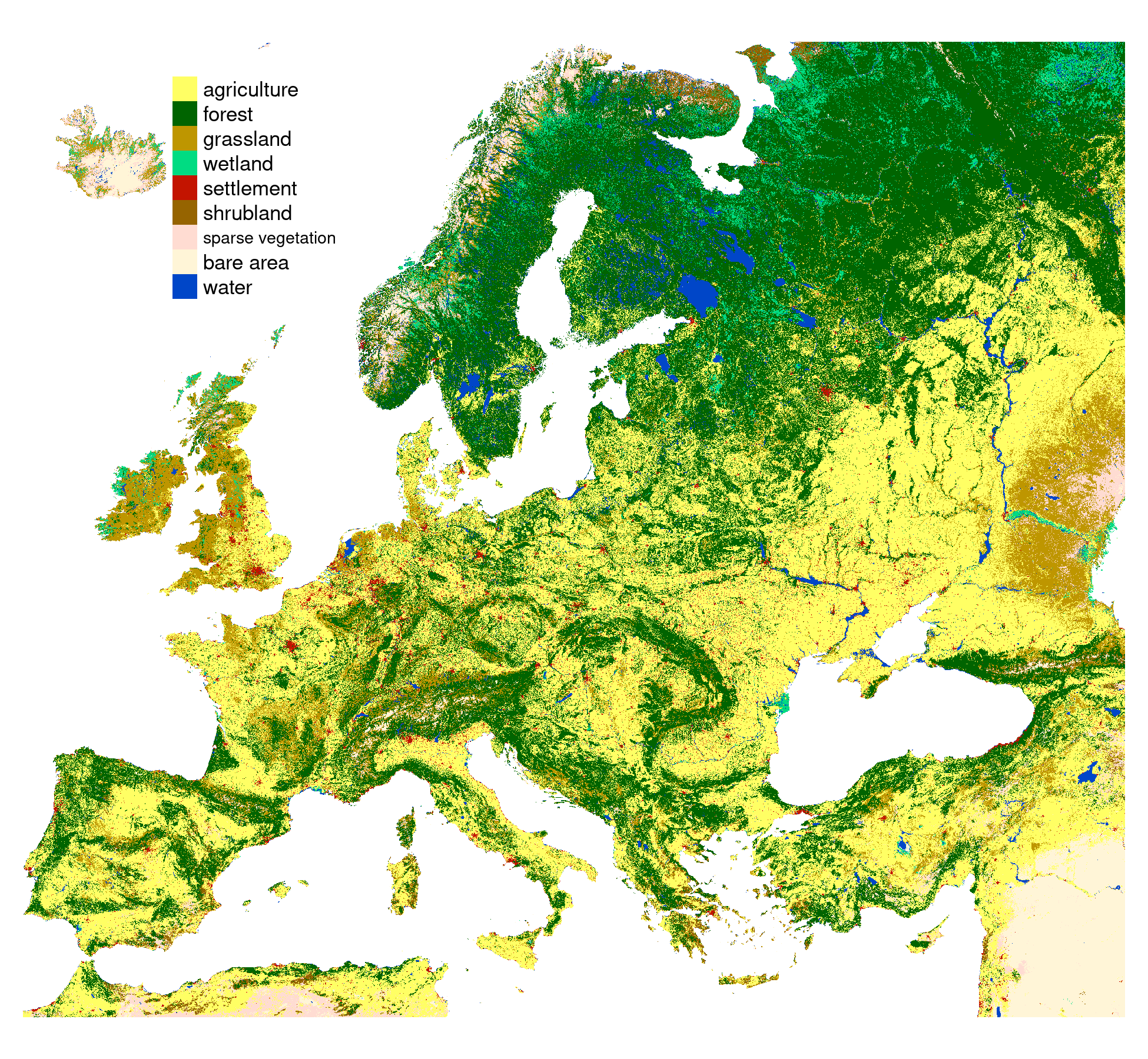
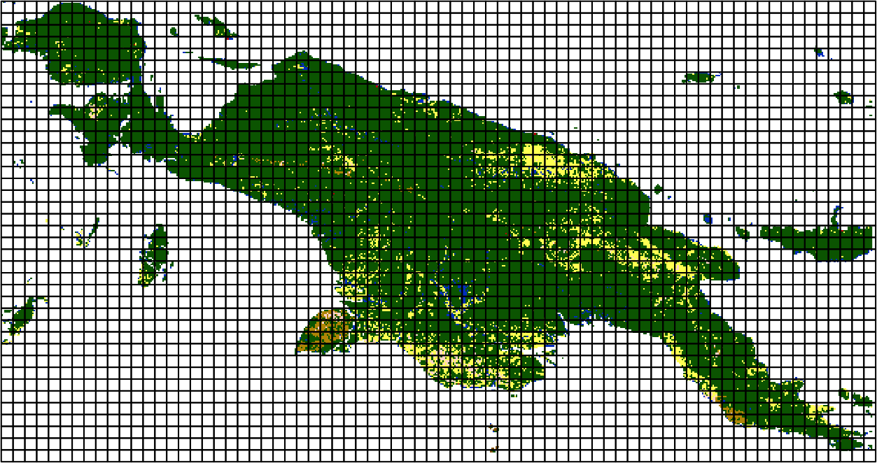
Example data
- Land cover data for the year 2016 from the CCI-LC project
- Simplified into nine main categories
Example data
- Land cover data for the year 2016 from the CCI-LC project
- Simplified into nine main categories
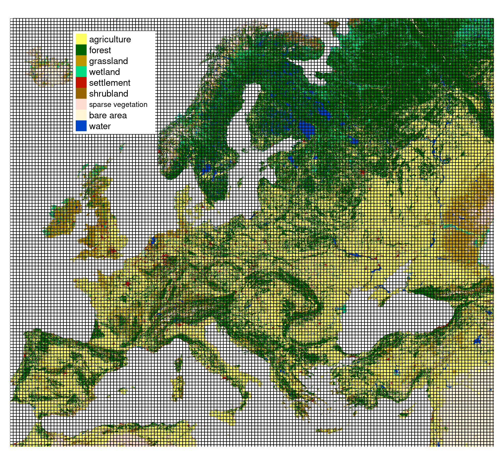
- Partitioned into 30 x 30 kilometers square blocks
- 13,909 categorical rasters (100x100 cells)
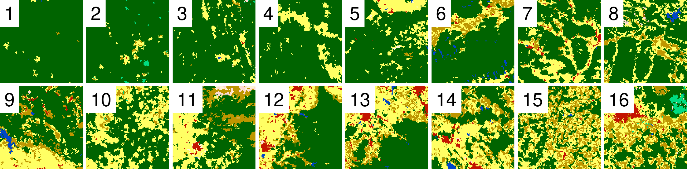
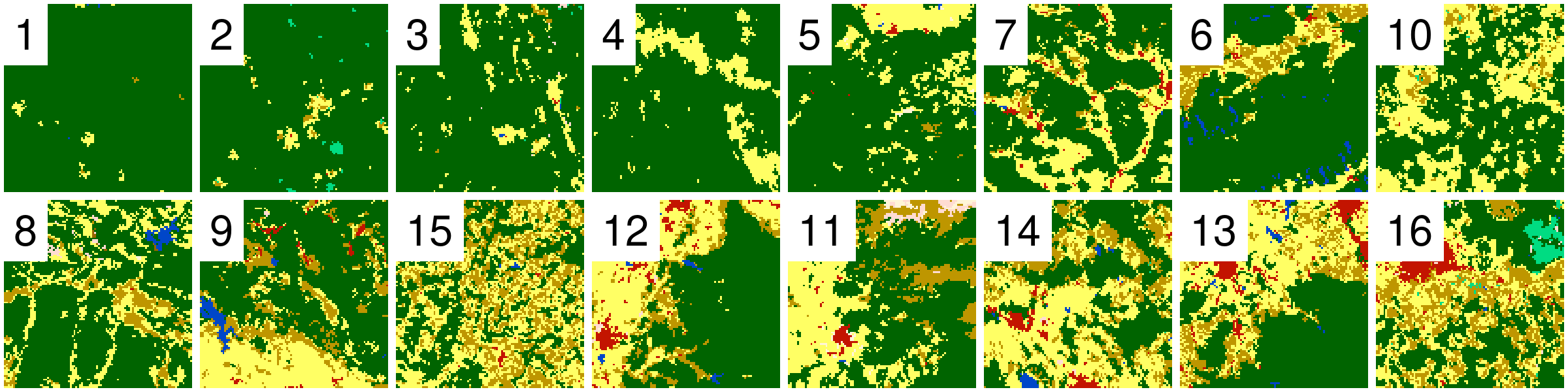
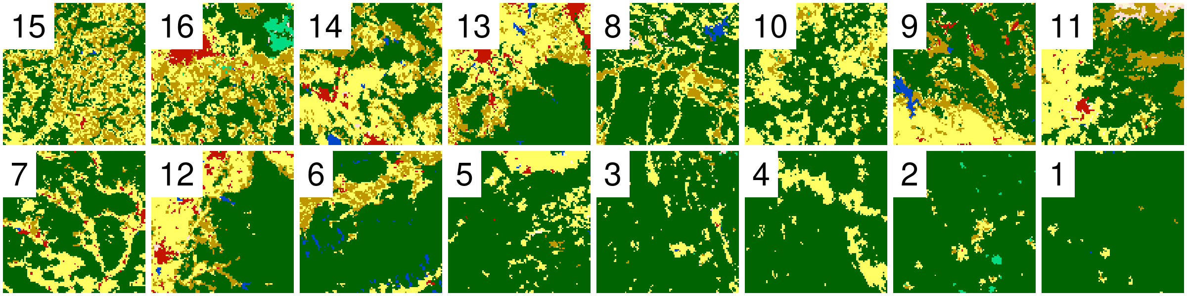
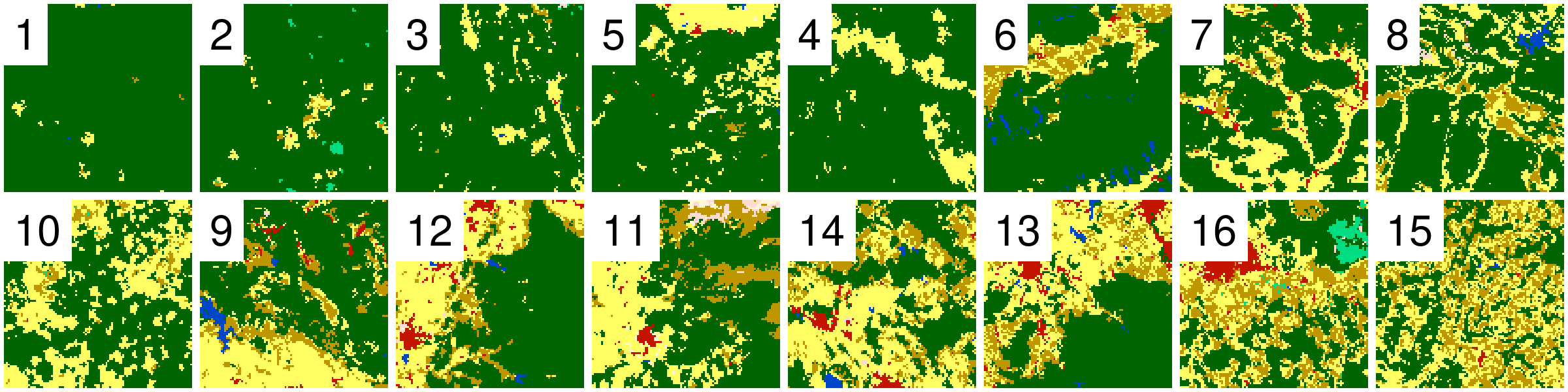
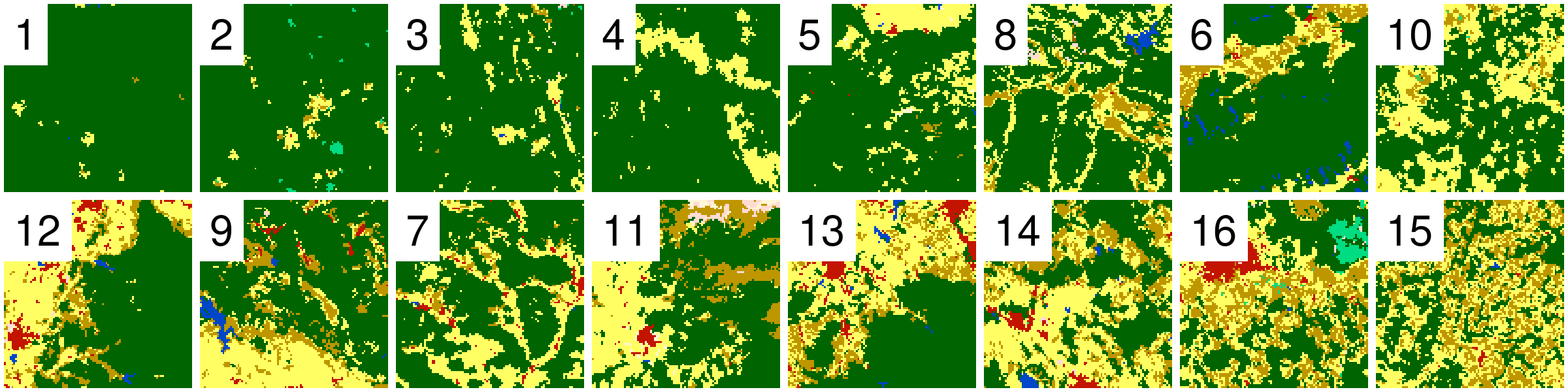
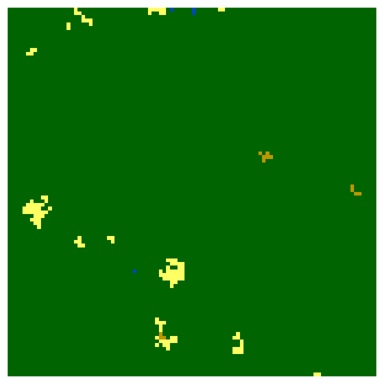
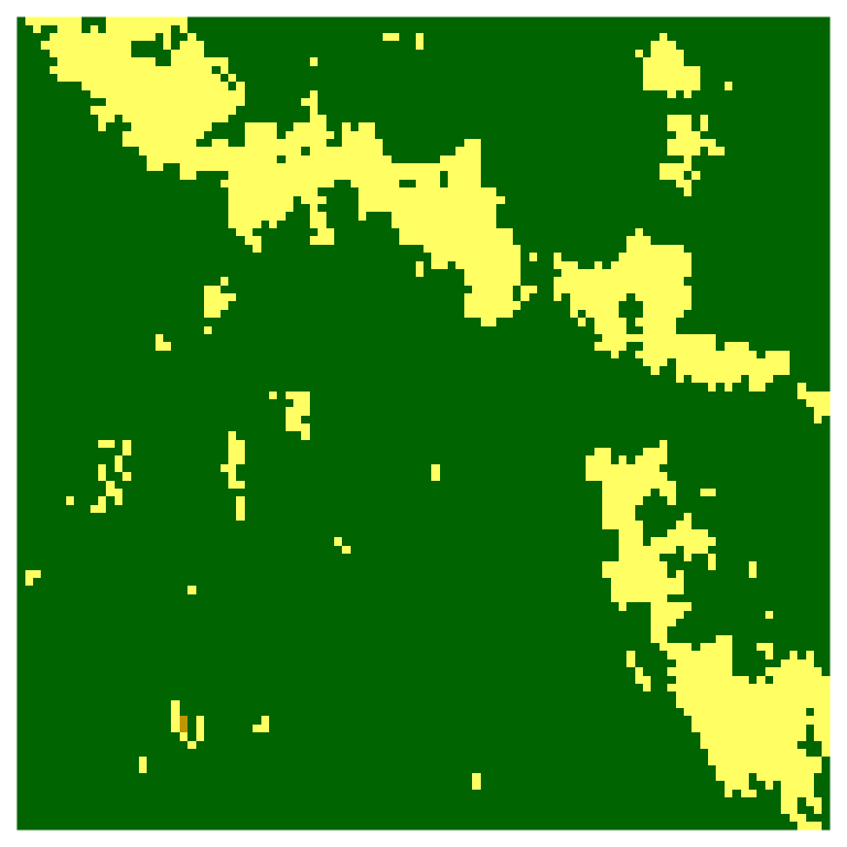
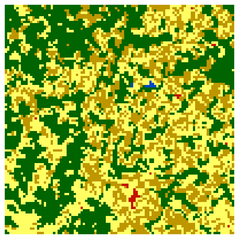
Example data
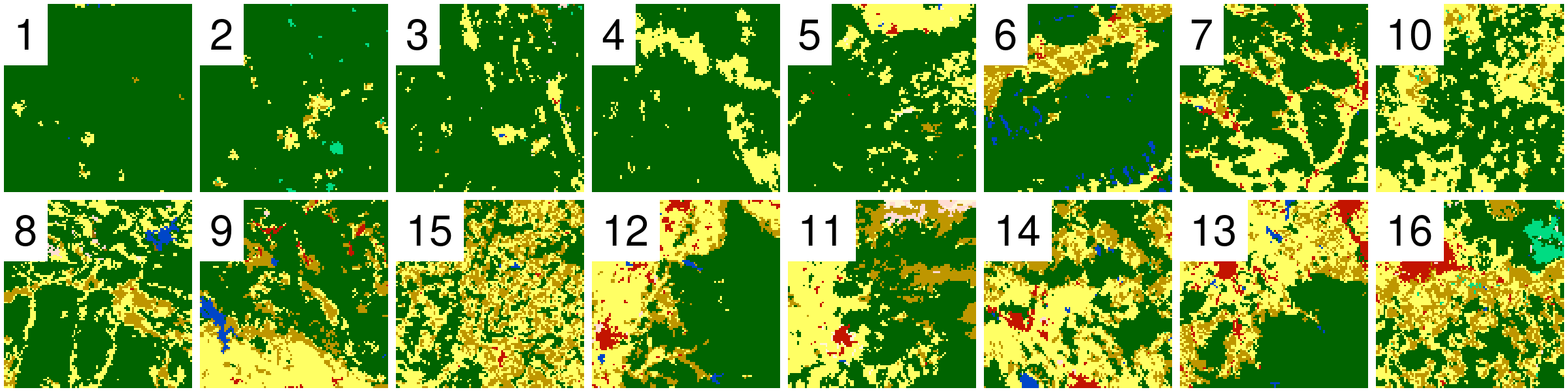
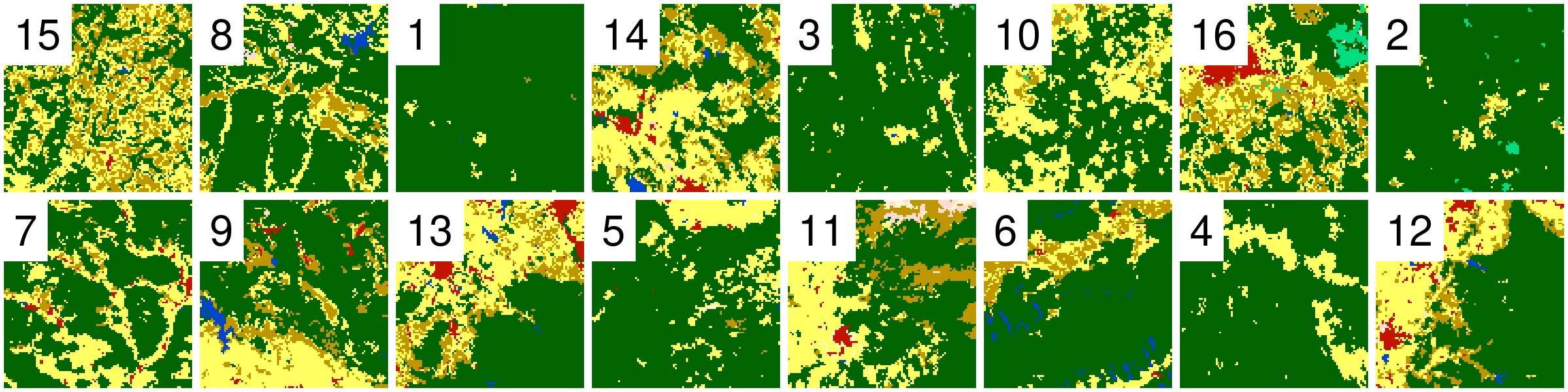
I randomely selected 16 rasters with different proportions of forest (green) areas:
Landscape metrics
- In the last 40 or so years, several hundred different landscape metrics were developed
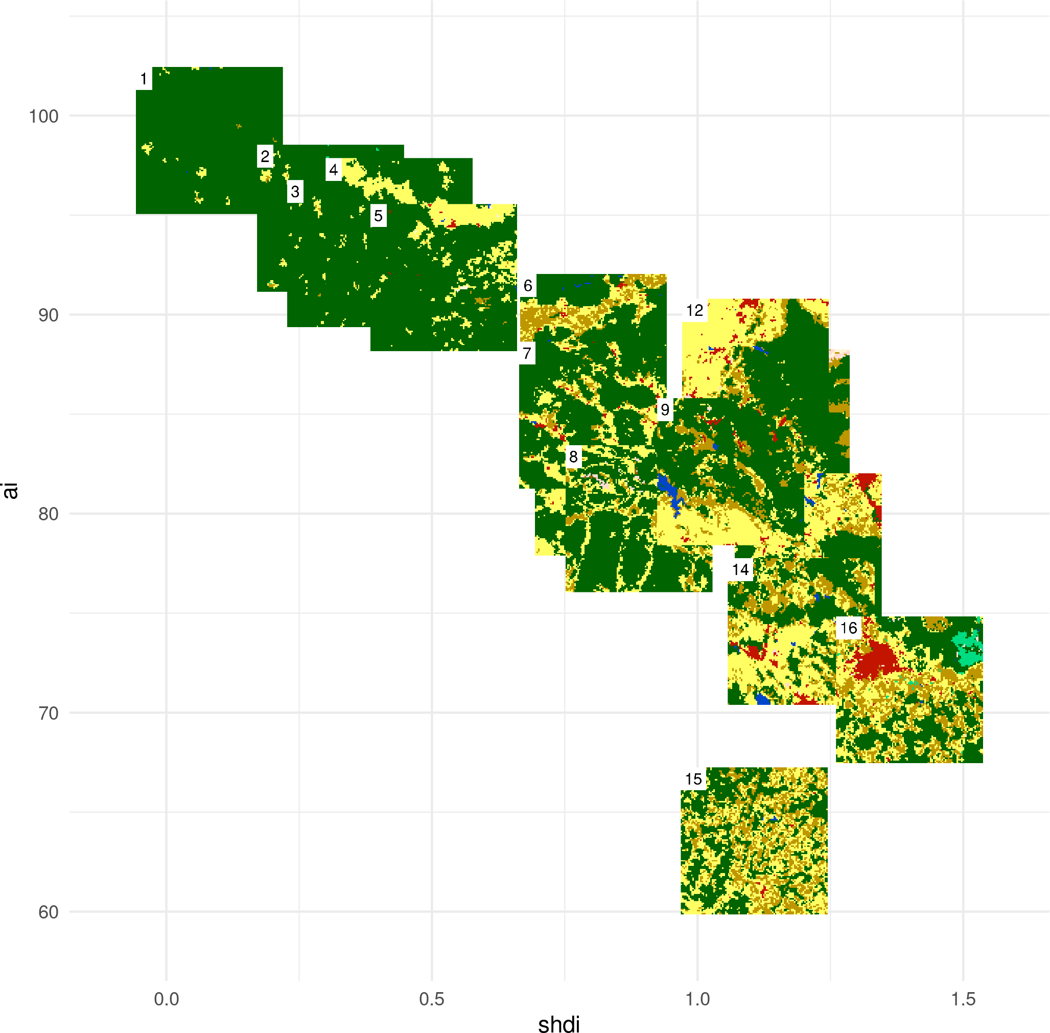
- SHDI - Shannon’s diversity index - takes both the number of classes and the abundance of each class into account
- AI - Aggregation index - from 0 for maximally disaggregated to 100 for maximally aggregated classes
SHDI:
AI:
Landscape metrics
- Problem no. 1: which of the hundreds of spatial metrics should we choose?
- Problem no. 2: many landscape metrics are highly correlated…
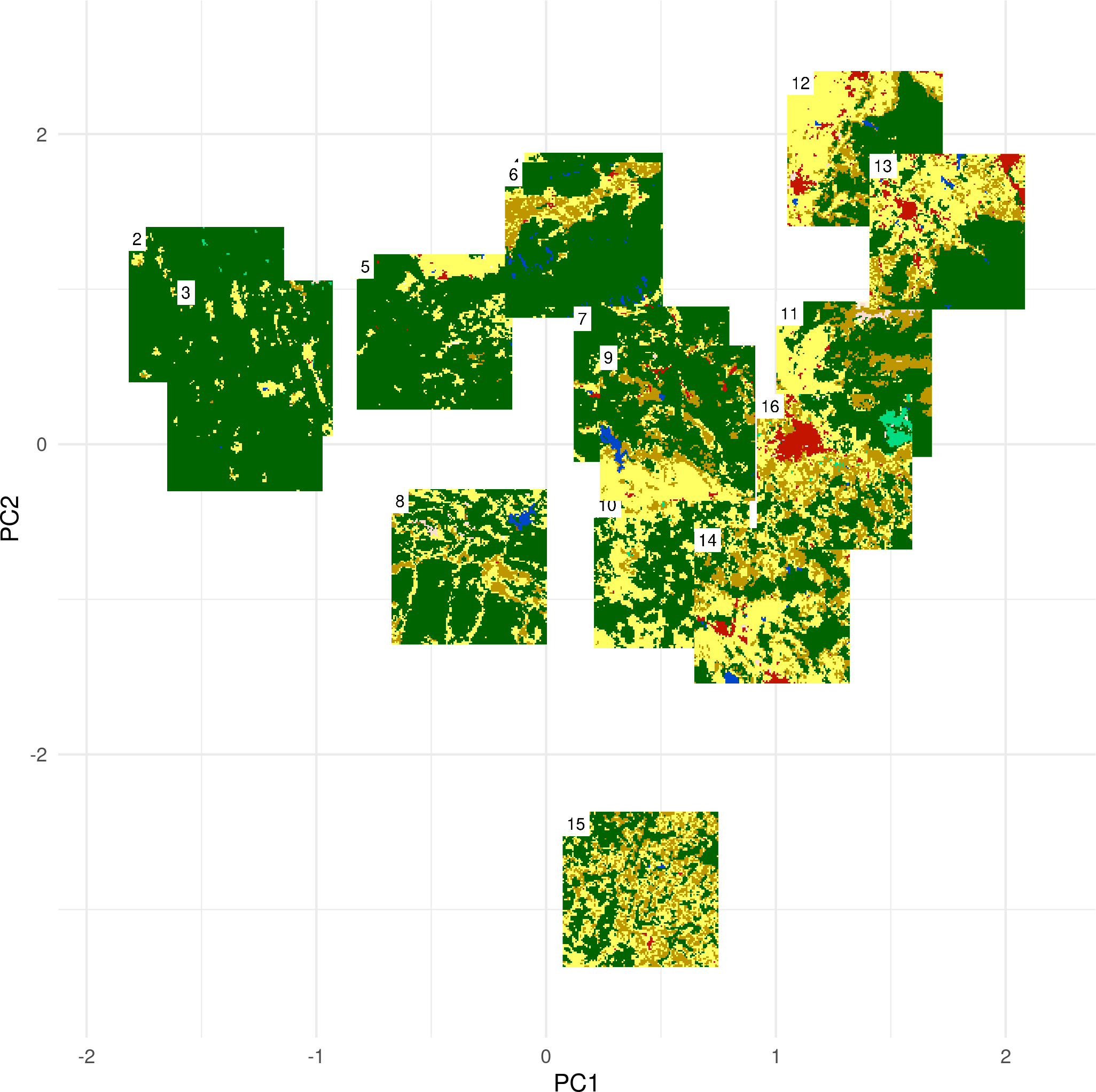
PCA of landscape metrics
- I performed a principal component analysis (PCA) using 17 landscape-level metrics:
| Type | Landscape-level metrics |
|---|---|
| Shape | PAFRAG; CONTIG AM; CONTIG RA |
| Aggregation | AI; CONTAG; IJI; PLATJ; PD; DIVISION; LPI |
| Connectivity | COHESION |
| Diversity | SHDI; SIDI; MSIDI; SHEI; SIEI; MSIEI |
- First two principal components explained ~71% of variability
PC1:
PC2:
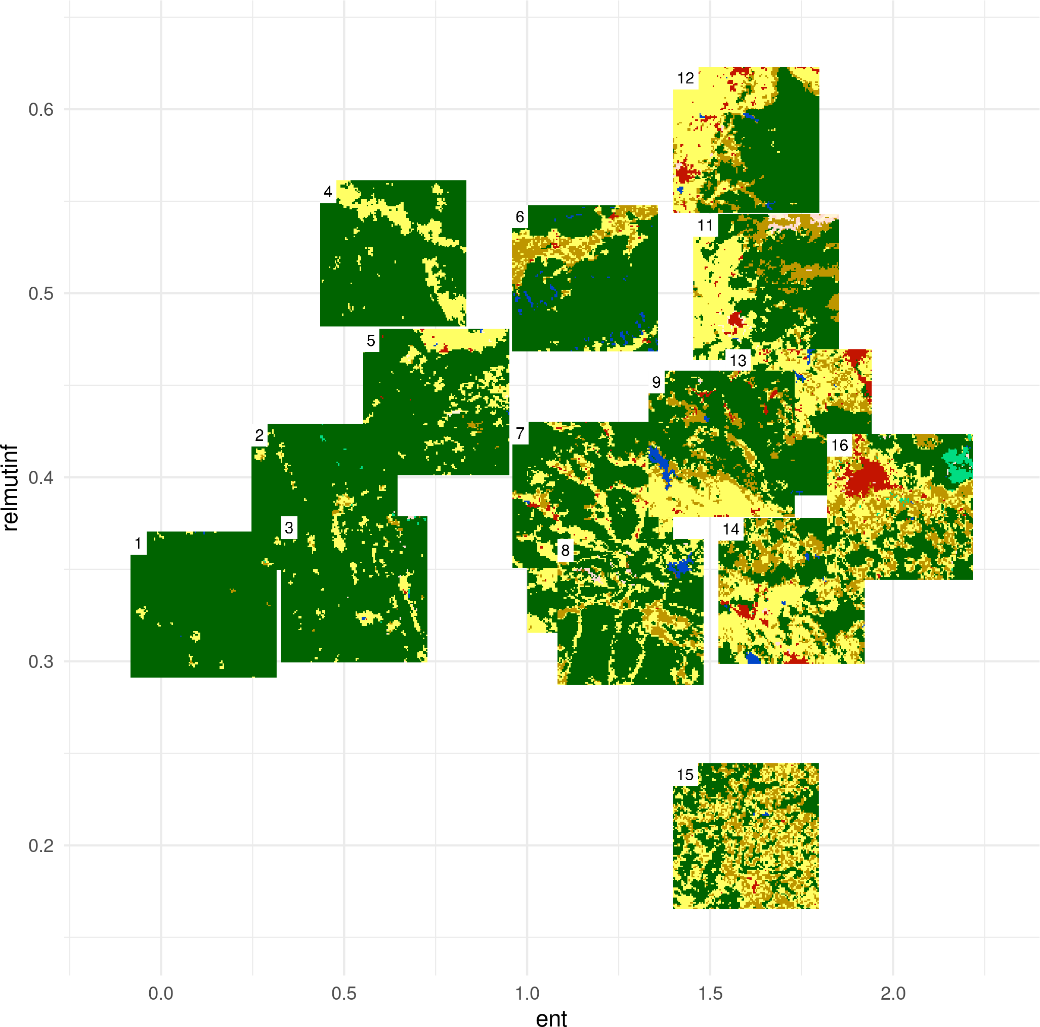
PCA of landscape metrics
The result allows to distinguish between:
- simple and complex rasters (left<->right)
- fragmented and consolidated rasters (bottom<->top)
However, there are still some problems here…
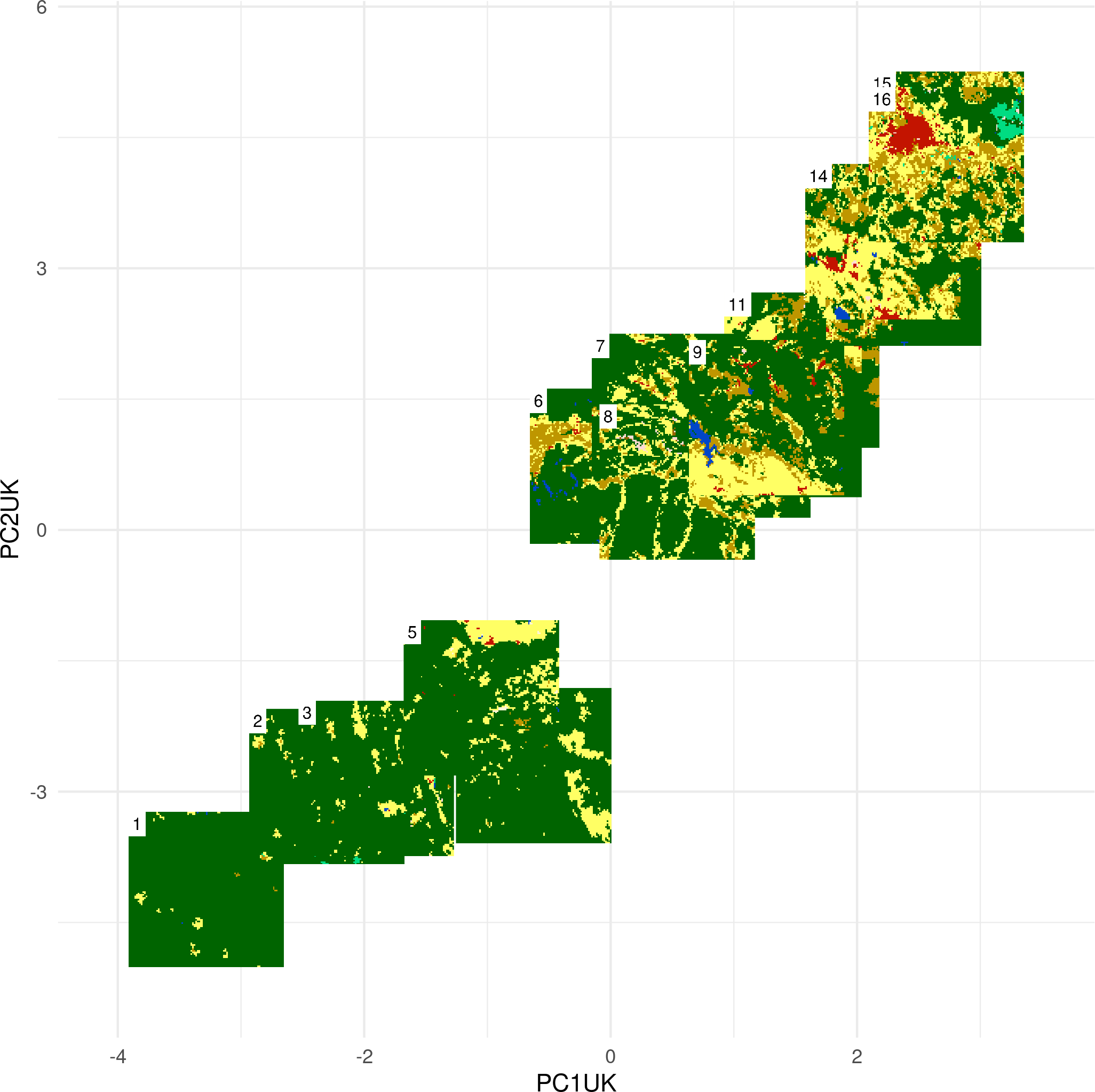
PCA of landscape metrics
- I performed a second PCA using data from the United Kingdom only
- Next, I predict the results on the data for the whole Europe
PC1:
PC2:
PCA of landscape metrics
Issues with the PCA approach:
- Each new dataset requires recalculation of both, landscape metrics and principal components analysis (PCA)
- Highly correlated landscape metrics are used
- PCA results interpretation is not straightforward
IT metrics
- Five information theory metrics based on a co-occurrence matrix exist (Nowosad and Stepinski, 2019, https://doi.org/10.1007/s10980-019-00830-x)
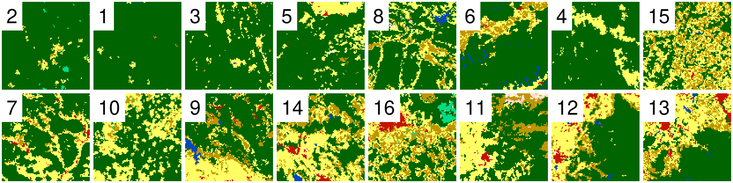
- Marginal entropy [H(x)] - diversity (composition) of spatial categories - from monothematic patterns to multithematic patterns
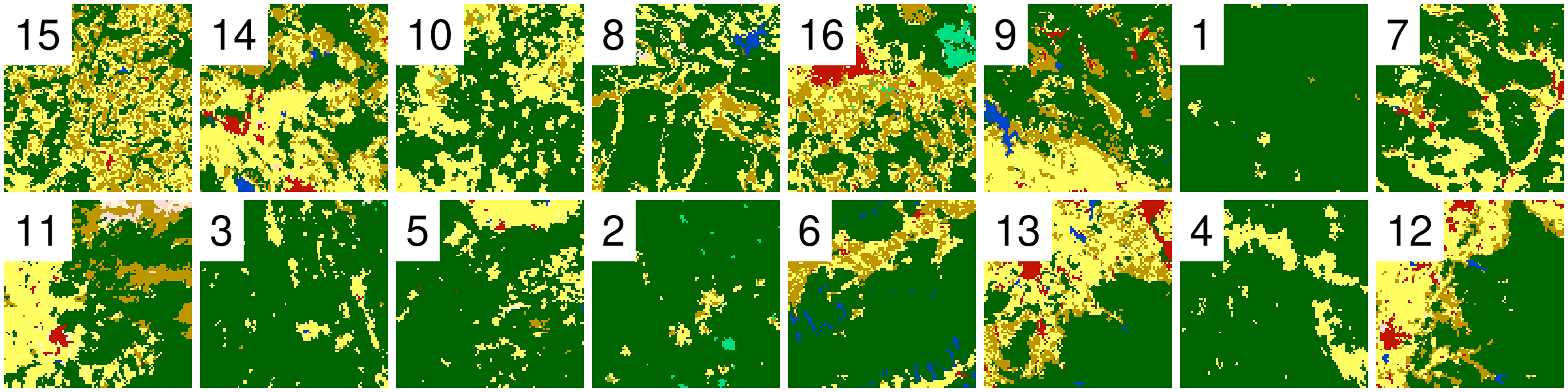
- Relative mutual information [U] - clumpiness (configuration) of spatial categories from fragmented patterns to consolidated patterns)
- H(x) and U are uncorrelated
Entropy:
Relative mutual information:
IT metrics
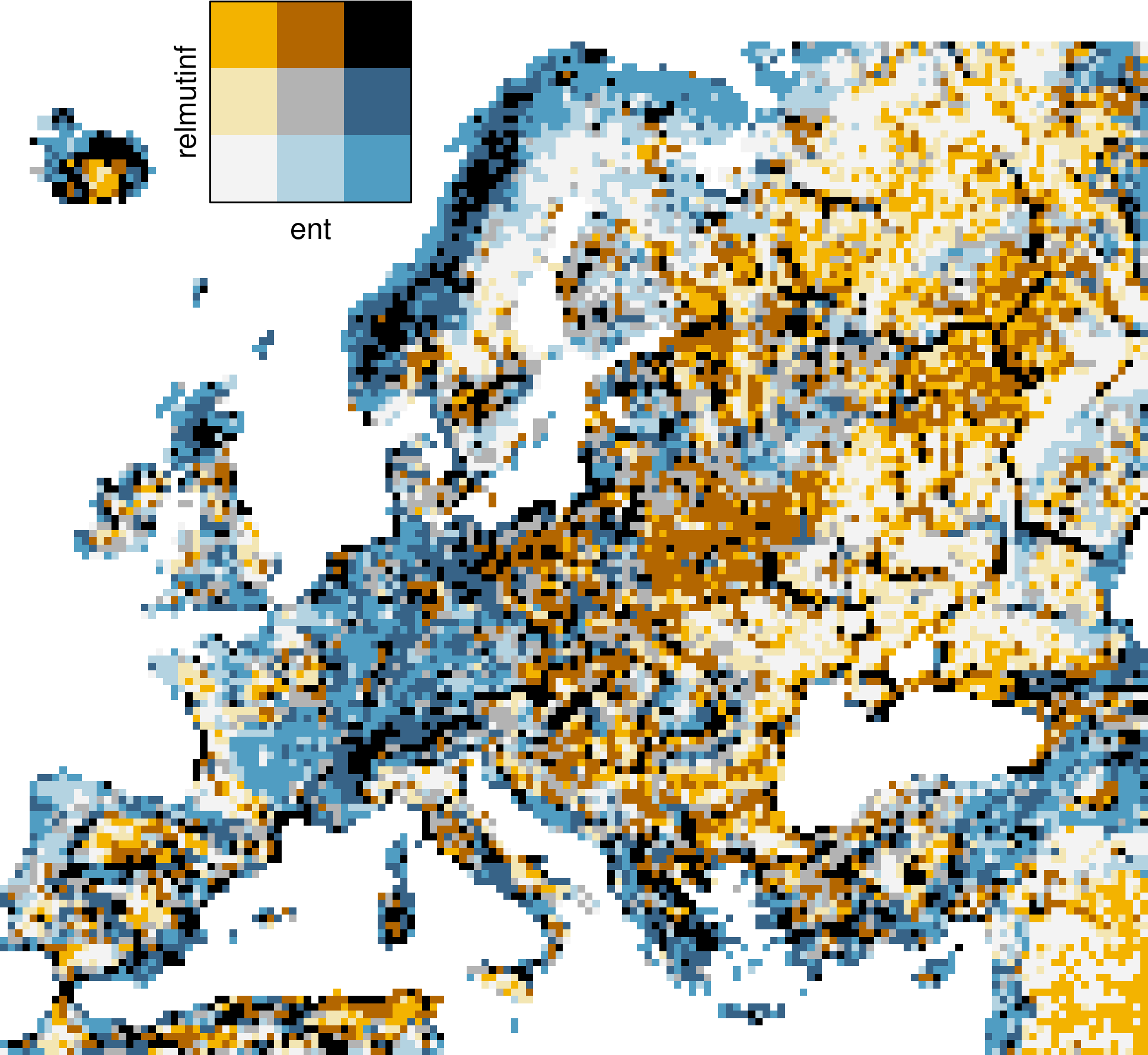
2D parametrization of categorical rasters’ configurations based on two weakly correlated IT metrics groups similar patterns into distinct regions of the parameters space
IT metrics - final results
Land cover data:
Parametrization using two IT metrics:
IT metrics
These metrics still leave some questions open…
- Relative mutual information is a result of dividing mutual information by entropy. What to do when the entropy is zero?
- How to incorporate the meaning of categories into the analysis?
Parametrization using two IT metrics:
Pattern-based spatial analysis
In recent years, the ideas of analyzing spatial patterns have been extended through an approach called pattern-based spatial analysis (Long in in. 2010; Cardille in in. 2010; Cardille in in. 2012; Jasiewicz i in. 2013; Jasiewicz i in. 2015).
The fundamental idea is to divide data into a large number of smaller areas (local landscapes).
Next, represent each area using a statistical description of the spatial pattern - a spatial signature.
Spatial signatures can be compared using a large number of existing distance or dissimilarity measures (Lin 1991; Cha 2007).
This approach enables spatial analyses such as searching, change detection, clustering, or segmentation.
Spatial signatures
Most landscape metrics are single numbers representing specific features of a local landscape.
Spatial signatures, on the other hand, are multi-element representations of landscape composition and configuration.

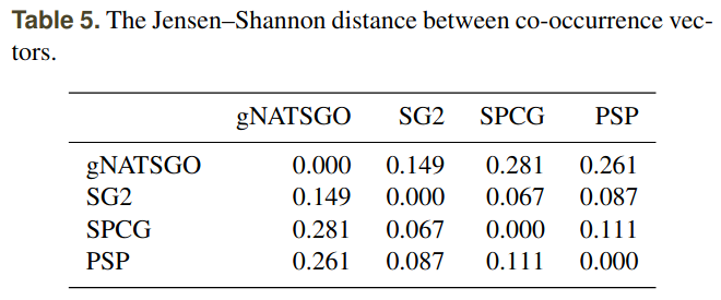
The basic signature is the co-occurrence matrix:
| agriculture | forest | grassland | water | |
|---|---|---|---|---|
| agriculture | 272 | 218 | 4 | 0 |
| forest | 218 | 38778 | 32 | 12 |
| grassland | 4 | 32 | 16 | 0 |
| water | 0 | 12 | 0 | 2 |
Spatial signatures
A spatial signature should allow simplification to the form of a normalized vector.

- Co-occurrence vector (cove):
| 272 | 218 | 4 | 0 | 218 | 38778 | 32 | 12 | 4 | 32 | 16 | 0 | 0 | 12 | 0 | 2 |
- Co-occurrence vector (cove):
| 136 | 218 | 19389 | 4 | 32 | 8 | 0 | 12 | 0 | 1 |
- Normalized co-occurrence vector (cove):
| 0.0069 | 0.011 | 0.9792 | 0.0002 | 0.0016 | 0.0004 | 0 | 0.0006 | 0 | 0.0001 |
Dissimilarity measures
Measuring the distance between two signatures in the form of normalized vectors allows determining dissimilarity between spatial structures.
| 0.0069 | 0.011 | 0.9792 | 0.0002 | 0.0016 | 0.0004 | 0 | 0.0006 | 0 | 0.0001 |
| 0.1282 | 0.0609 | 0.8105 | 0.0002 | 0.0002 | 0.0001 | 0 | 0 | 0 | 0 |
\[JSD(A, B) = H(\frac{A + B}{2}) - \frac{1}{2}[H(A) + H(B)]\]
Jensen-Shannon distance between the above rasters: 0.0684
Dissimilarity measures
Measuring the distance between two signatures in the form of normalized vectors allows determining dissimilarity between spatial structures.

| 0.0069 | 0.011 | 0.9792 | 0.0002 | 0.0016 | 0.0004 | 0 | 0 | 0 | 0 | 0 | 0.0006 | 0 | 0 | 0.0001 |
| 0.2033 | 0.1335 | 0.2944 | 0.1747 | 0.0562 | 0.1307 | 0.0035 | 0.0002 | 0.0004 | 0.0015 | 0.0007 | 0.0005 | 0 | 0 | 0.0005 |
\[JSD(A, B) = H(\frac{A + B}{2}) - \frac{1}{2}[H(A) + H(B)]\]
Jensen-Shannon distance between the above rasters: 0.444
Pattern-based spatial analysis
Knowing the distance between spatial signatures can be used in several contexts (Nowosad, 2021, 10.1007/s10980-020-01135-0):
one-to-many
finding similar spatial structures
one-to-one
quantitative assessment of changes in spatial structures
many-to-many
clustering similar spatial structures
One-to-many
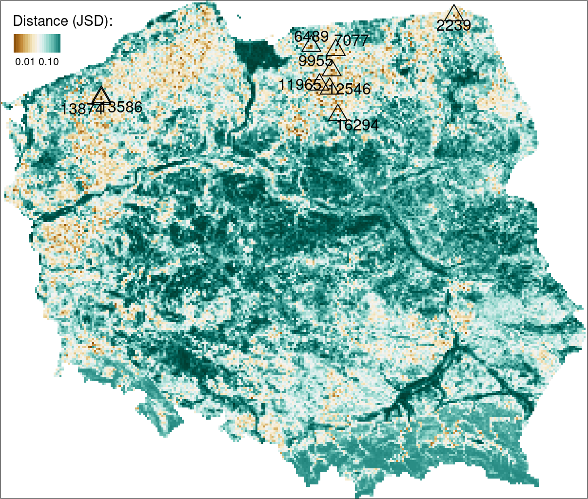
Finding areas with similar topography to the Suwalski Landscape Park.
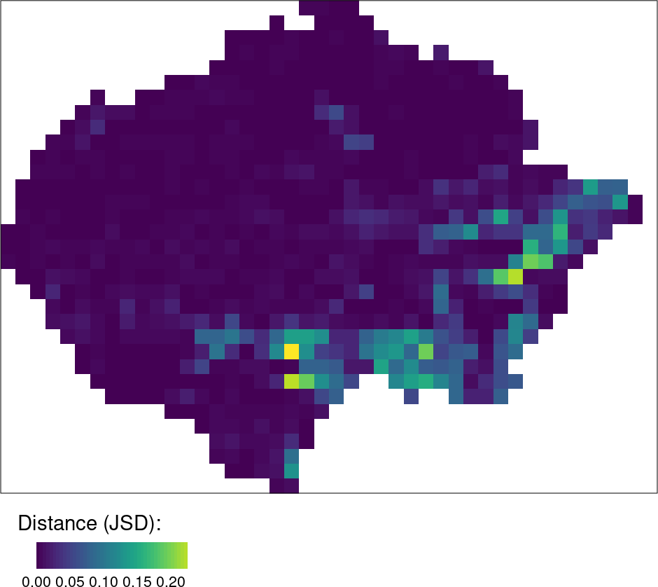
One-to-one
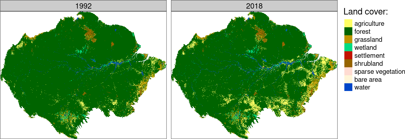
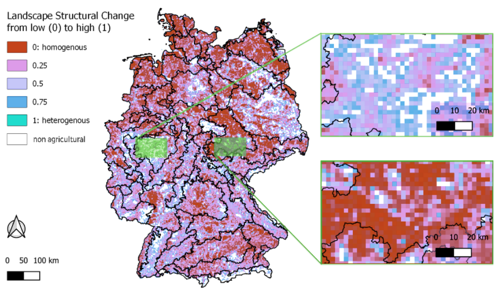
The map above shows that many areas in the Amazon have undergone significant land cover changes between 1992 and 2018.
The challenge now is to determine which areas have changed the most.
One-to-one
Areas with the greatest change have the highest dissimilarity values.
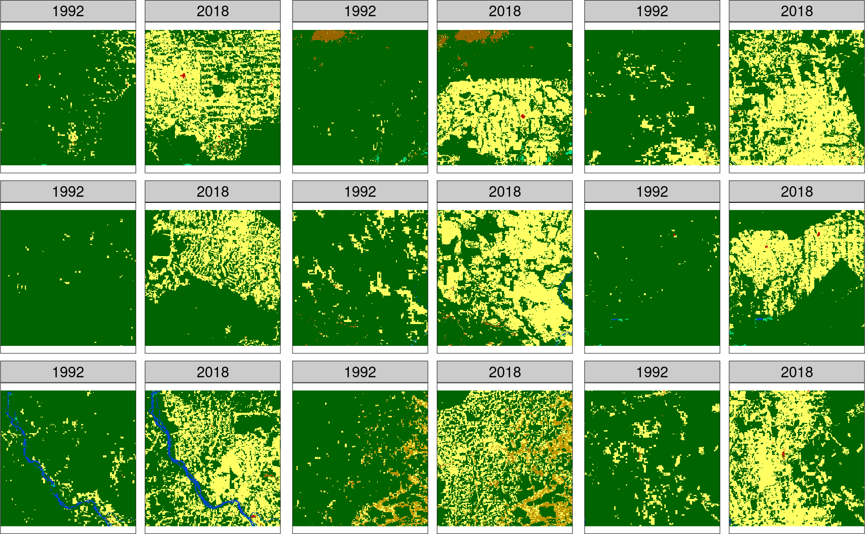
Importantly, changes in both category and spatial configuration are measured.
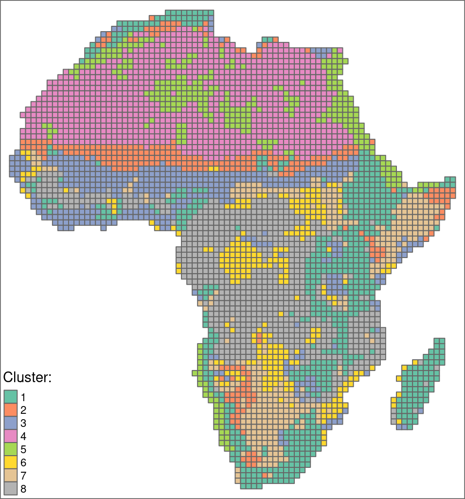
Many-to-many
Areas in Africa with similar spatial structures for two themes have been identified - land cover and landforms.
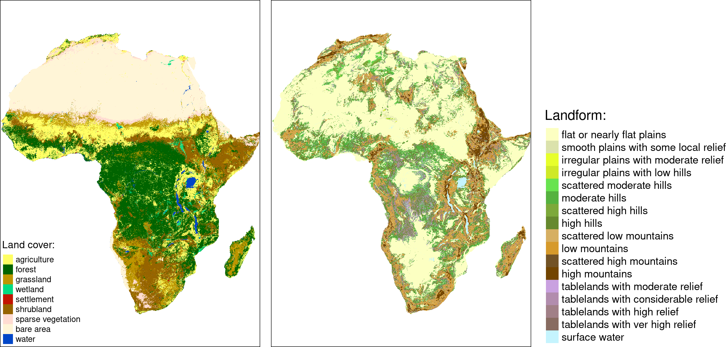
Many-to-many
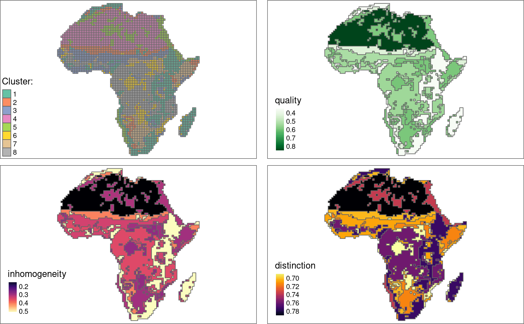
The quality of each cluster can be assessed using metrics:
- Intra-cluster heterogeneity - determines distances between all landscapes within a group
- Inter-cluster isolation - determines distances between a given group and all others
Examples of applications
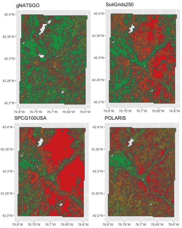
Using spatial signatures to compare and evaluate digital soil maps (Rossiter et al., 2022, 10.5194/soil-8-559-2022)
Changes in spatial patterns resulting from the inclusion of small woody elements in land use maps (Golicz et al., 2021, 10.3390/land10101028)
Non-categorical rasters
WorldClim version 2.1 climate data
for 1970-2000
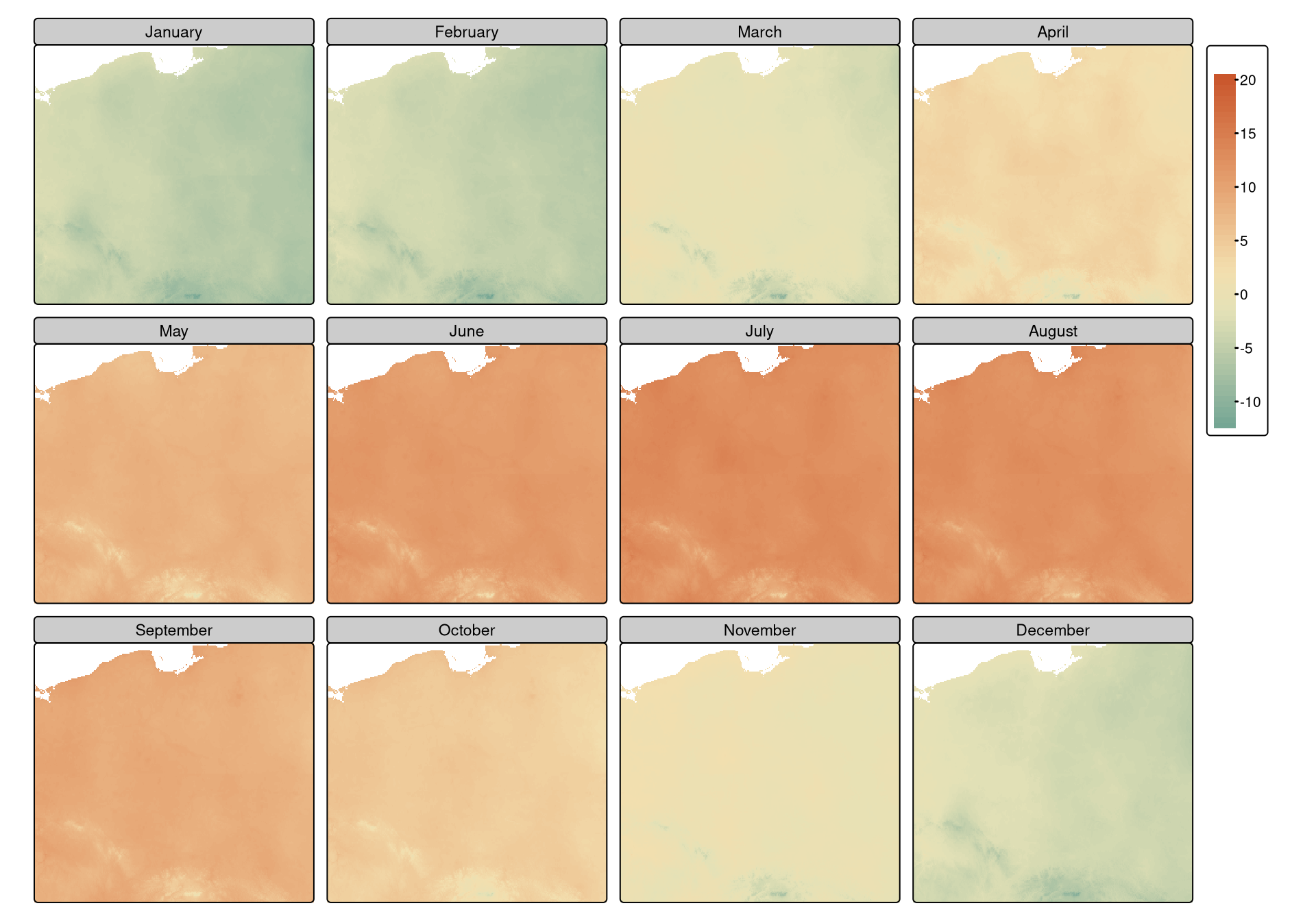
CMIP6 downscaled future climate projection for 2061-2080 [model: CNRM-ESM2-1; ssp: “585”]
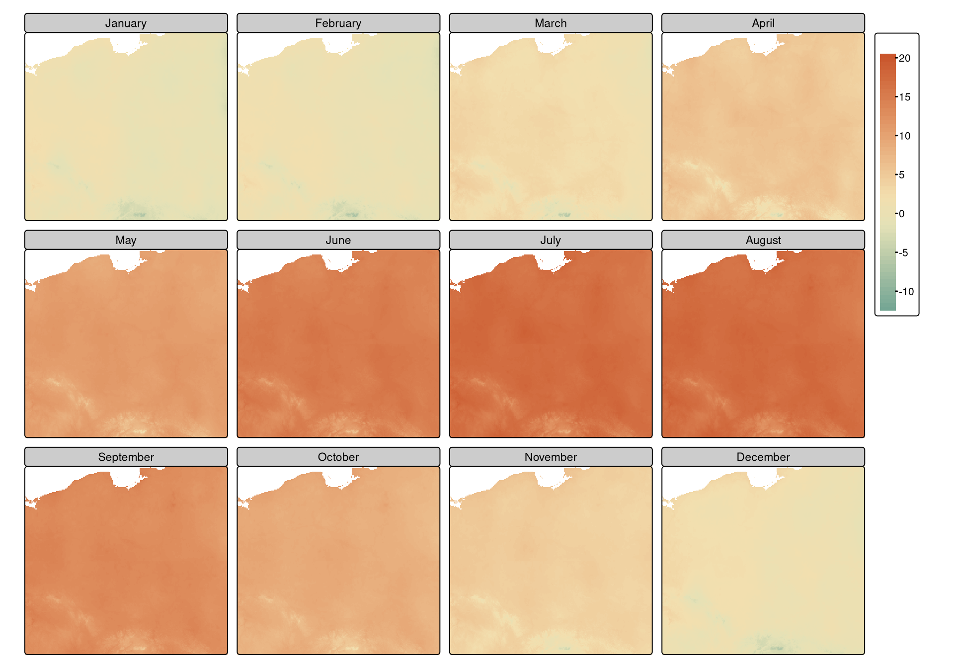
Minimum temperature (°C)
{spquery}
https://jakubnowosad.com/spquery/
How to find and compare areas with similar spatial patterns in non-categorical rasters (e.g., raster time-series)?
Search
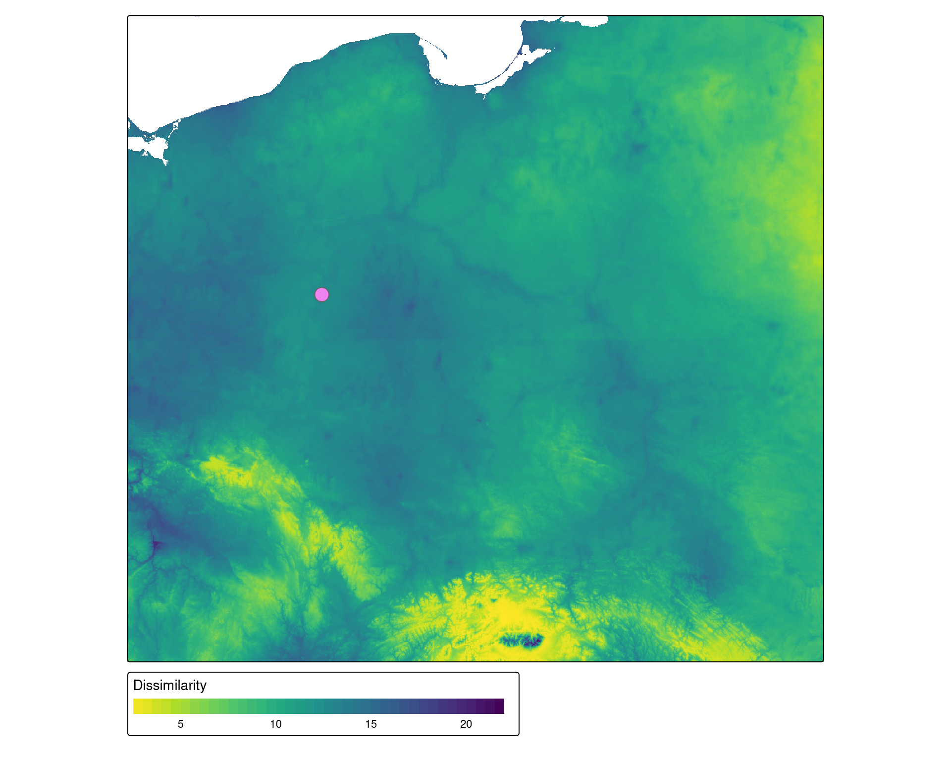
Compare
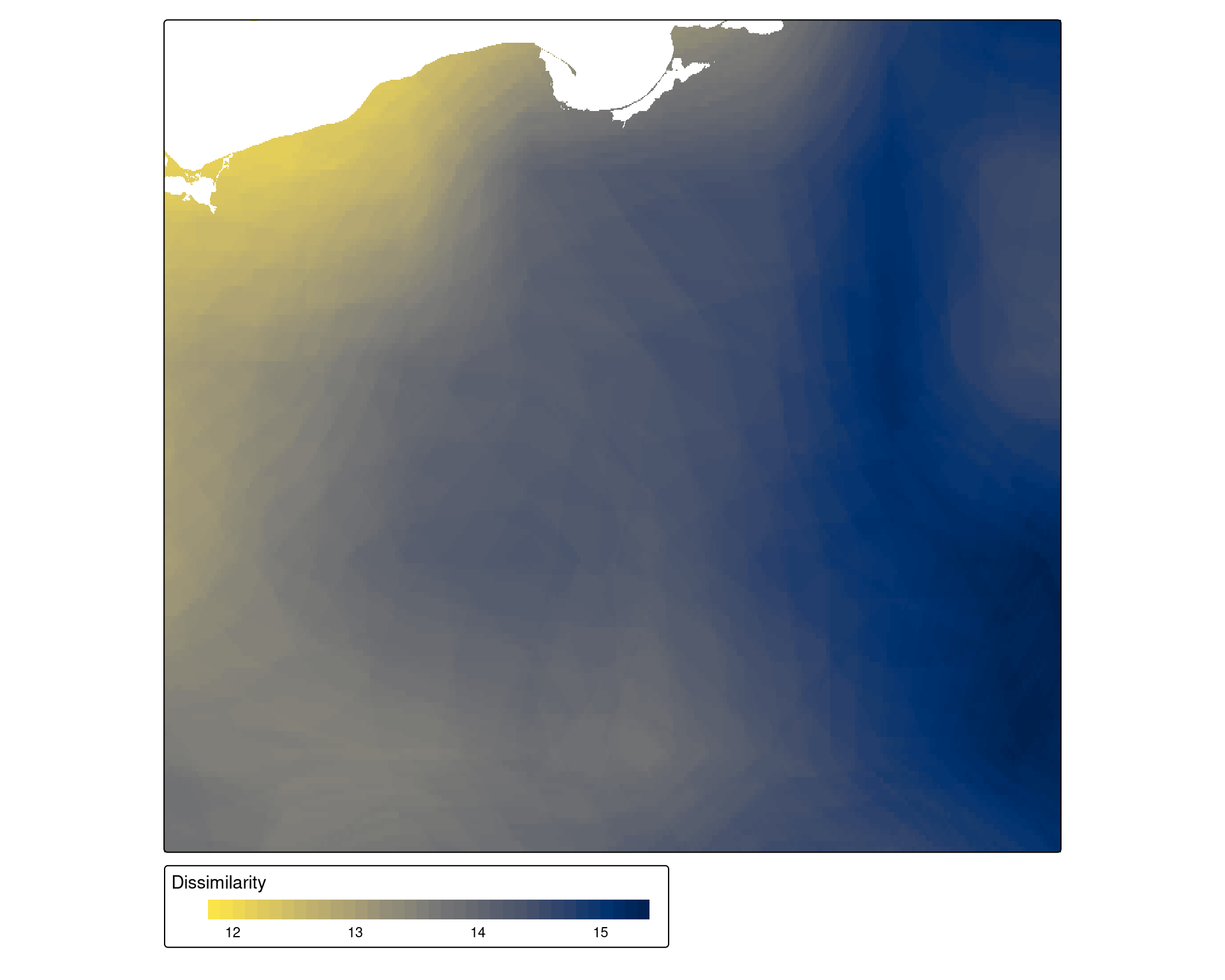
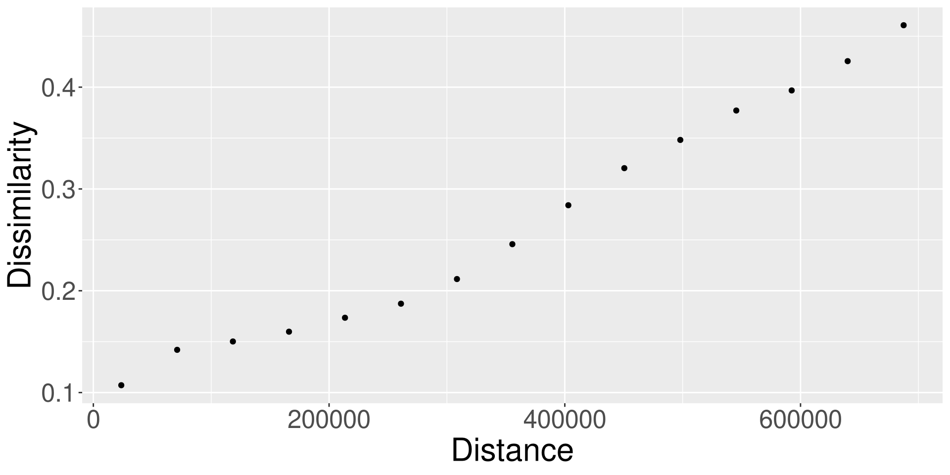
{patternogram}
https://jakubnowosad.com/patternogram/, https://jakubnowosad.com/ecem-2023
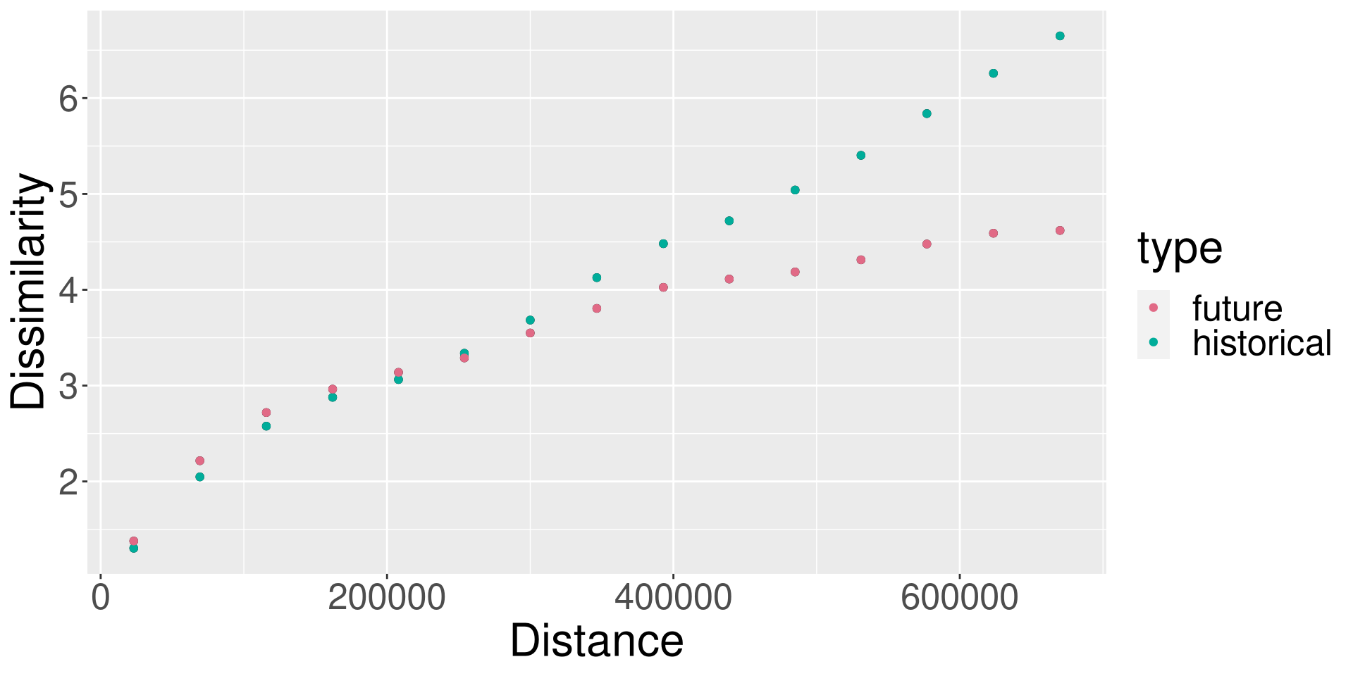
How to detect and describe a range of spatial similarity (spatial autocorrelation) for multiple variables?
It can be used to:
- explore spatial autocorrelations of predictors in machine learning models
- detect spatial autocorrelation in various data structures
- compare the spatial autocorrelation of variables over time
- investigate spatial autocorrelation of categorical spatial patterns
{patternogram}
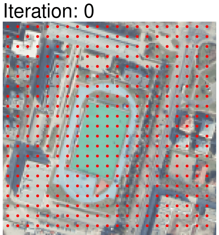
{supercells}
https://jakubnowosad.com/supercells/, https://jakubnowosad.com/foss4g-2022/
supercells: an extension of SLIC (Simple Linear Iterative Clustering; Achanta et al. (2012), doi:10.1109/TPAMI.2012.120) that can be applied to non-imagery geospatial rasters that carry:
- pattern information (co-occurrence matrices)
- compositional information (histograms)
- time-series information (ordered sequences)
- other forms of information for which the use of Euclidean distance may not be justified
Segmentation/regionalization: partitioning space into smaller segments while minimizing internal inhomogeneity and maximizing external isolation
A way to improve the output and reduce the cost of segmentation.
{supercells}
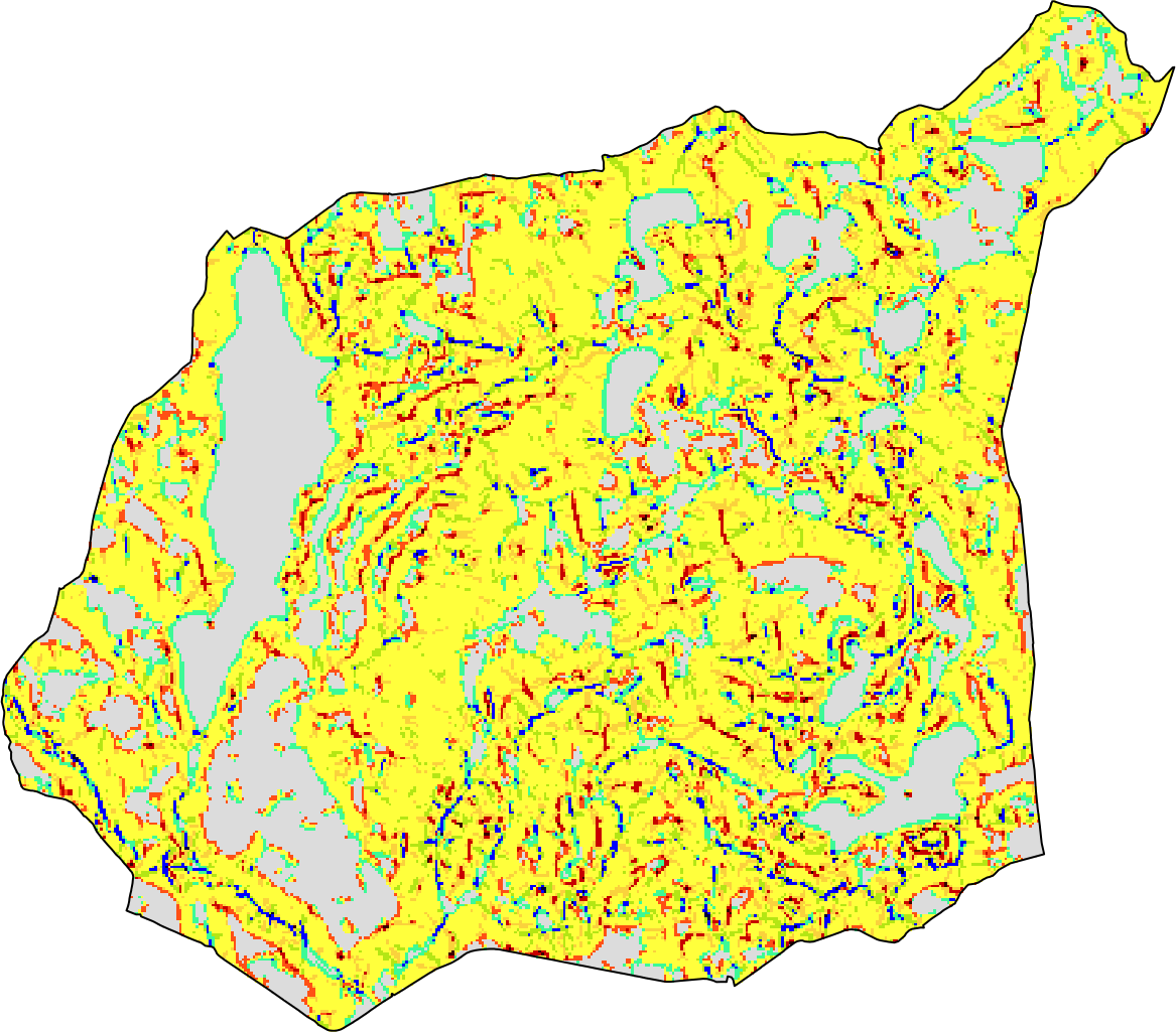
Great Britain. WorldClim gridded climate data was normalized to be between 0 and 1.
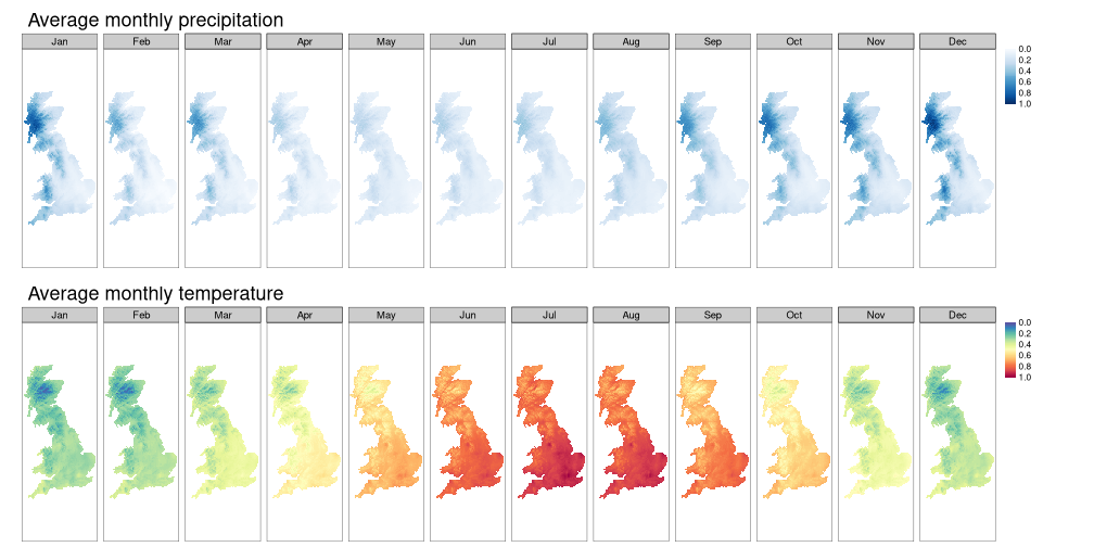
The goal: to regionalize Great Britain’s climates
{supercells}
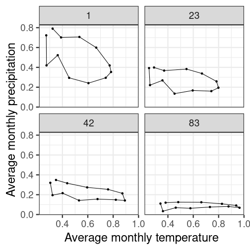
Extended SLIC workflow uses the dynamic time warping (DTW) distance function rather than the Euclidean distance.
{supercells}
Extended SLIC: a more homogeneous regionalization.
Original SLIC: more isolated regions.
| SLIC | Inhomogeneity | Isolation |
|---|---|---|
| extended | 0.30 | 0.59 |
| original | 0.37 | 0.75 |
The raster of time series compressed from 24 dimensions to three principal components preserving 99% of variability.