Moving beyond pattern-based analysis: Additional applications of GeoPAT 2

This is the sixth and the last blog post in the series introducing GeoPAT 2 - a software for pattern-based spatial and temporal analysis. In the previous one we presented the pattern-based spatial segmentation - a method for creating regions of homogeneous patterns. Here, we will mention other pattern-based methods and show some examples of how you can use pieces of GeoPAT 2 in your own workflow.

Introduction

GeoPAT 2 gives its users a lot of freedom, having a large number of possible workflows:

Outline of the GeoPAT 2 architecture

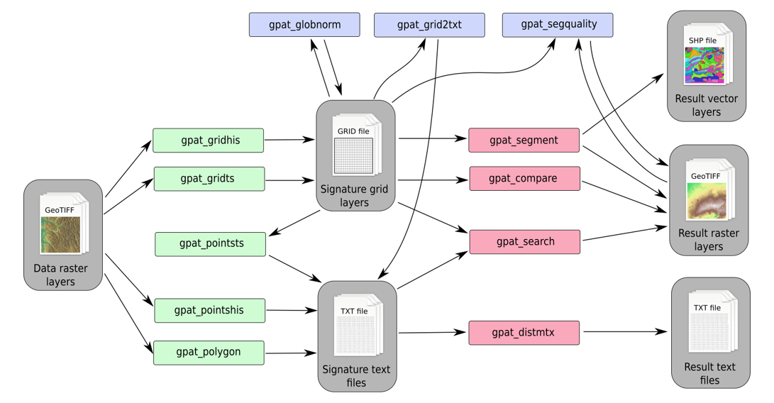
Some of them can consist of only one step, while others require several steps. However, that is not the end of GeoPAT 2 capabilities - it is also possible to extract spatial signature or calculate distance matrix and use these outputs in further analysis outside of GeoPAT 2. For example, you can cluster areas of similar patterns or use machine learning methods to find numerical relationships between patterns descriptors and other variables. Finally, there are several experimental features of GeoPAT 2, including a set of methods for analysis of spatiotemporal data.

We are going to use land cover data of Australia from the year 2015 and TNC’s terrestrial ecoregions of the same area as examples in this blog post. To follow the subsequent calculations, you need to download these datasets, cci_lc2015.tif and tnc_terr_ecoregions.tif, and install GeoPAT 2. Some examples also use rgeopat2 - an R package with additional functions for GeoPAT 2:

install.packages("rgeopat2")

Extracting information about spatial patterns

Most of the GeoPAT 2 modules depends on spatial information about patterns in the form of signatures. We can then find the most similar signatures (search), compare local signatures (comparison), or merge areas with similar signatures (segmentation). This information can be also used outside of GeoPAT 2 - it is possible to fit a spatial pattern information to your own workflow.

There are three main ways to extract information about spatial patterns. The first one extracts information from a regular grid of motifels. In the example below, we create a grid of motifels with information about the composition of land cover categories (-s prod). Next, using gpat_grid2txt we convert the output grid file into a text file that can be read by standard software, such as R, Python, Excel.

gpat_gridhis -i cci_lc2015.tif -o patterns2015.grd -s prod -z 200 -f 200
gpat_grid2txt -i patterns2015.grd -o patterns2015.txt

The second one extracts a spatial pattern information based on point coordinates within the given buffer. Below, we extract a land cover composition (Cartesian product) of a square area of 30 by 30 pixels (9km by 9km) around Australia’s capital - Canberra:

gpat_pointshis -i cci_lc2015.tif -o patterns_pts.txt -s prod -z 30 -x 1370000 -y -4050000

The third one involves extracting information about spatial patterns using irregular polygons with gpat_polygon. Let’s say, we are interested in extracting land cover composition in each of TNC’s terrestrial ecoregions in Australia. (Due to large sizes of some ecoregions, the below calculation can require about 16GB RAM available.)

gpat_polygon -i cci_lc2015.tif -e tnc_terr_ecoregions.tif -o patterns_poly.txt -s prod

To ease some of the non-standard GeoPAT 2 operations we created an R package called rgeopat2.

library(rgeopat2)

Its function gpat_read_txt() reads the output text from GeoPAT 2 and formats it in a convinent way:

patterns_poly = gpat_read_txt("patterns_poly.txt")

Example of two lines from the gpat_read_txt() output

	X1	X2	X3	X4	X5	X6	X7	X8	X9	X10	X11	X12	X13	X14	X15	X16	X17	X18	X19	X20	X21	X22	cat
1	0.00	0.00	0	0.00	0.00	0.00	0.00	0.00	0.00	0	0.00	0	0.00	0.00	0.00	0.00	0	0.00	0.00	0.00	0	1.00	0
34	0.00	0.00	0	0.00	0.00	0.00	0.00	0.00	0.00	0	0.00	0	0.00	0.00	0.54	0.45	0	0.00	0.00	0.00	0	0.00	10072

The last column in this table, cat, represents the id of the terrestrial ecoregion, while the rest of the columns are the land cover categories. For example, cat 0 is an ocean and 100% of its area is covered by water (class X22), while cat 10072, Gibson Desert, is located in the middle of the continent and is covered by grassland (X15) and sparse vegetation (X16).

Visualize spatial grids

Creating a grid of motifels is a basic task in many pattern-based analyses, which also includes selecting a size of the motifels.

gpat_gridhis -i cci_lc2015.tif -o patterns2015.grd -s prod -z 200 -f 200

To ease selection of a motifels’ size, we can use another function from the rgeopat2 package gpat_create_grid(). It takes a header output of the gpat_gridhis and produces a vectorized grid.

my_grid = gpat_create_grid("patterns2015.grd.hdr")

Now, you can impose it on top of your map to make a better decision about a motifel size.

A grid of motifels of 60 by 60 km imposed on the top of a land cover raster map

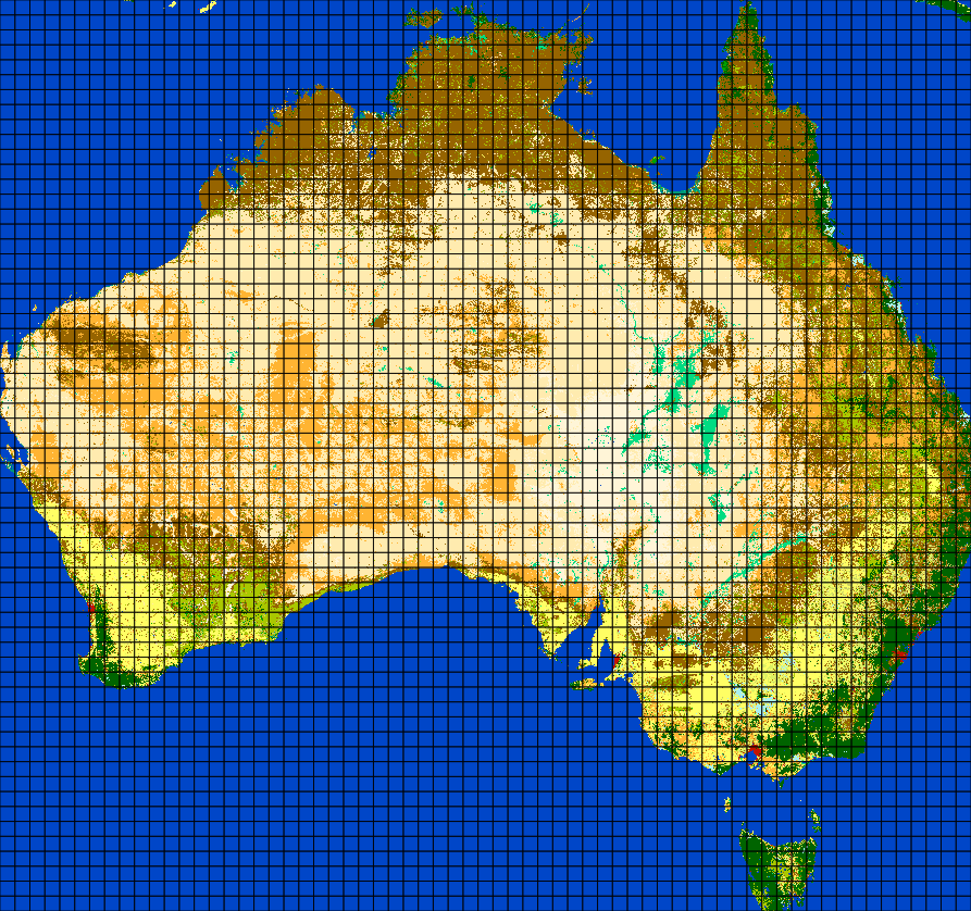
This function also can be used to analyze and present the results. One of the examples here is to extract information about spatial patterns from a grid using gpat_grid2txt, read it to R with gpat_read_txt() and finally merge it with spatial data.

library(sf)
library(dplyr)
patterns2015 = gpat_read_txt("patterns2015.txt")
my_patterns = bind_cols(my_grid, patterns2015)

The output of this operation is a spatial object (grid of motifels) with attributes about land cover composition.

Spatial pattern-based clustering

Extracting spatial signatures is not the end of the GeoPAT 2 capabilities. You can also calculate similarity matrices between motifels, points, or polygons using gpat_distmtx. It accepts outputs from gpat_grid2txt, gpat_pointshis, or gpat_polygon and returns a CSV file containing a similarity matrix - also known as a distance matrix. Below, we focus on the output from gpat_grid2txt. Read the GeoPAT 2 manual to see examples of clustering based on the output of gpat_pointshis and gpat_polygon.

gpat_distmtx -i patterns2015.txt -o similarity2015.csv

The output, similarity2015.csv, can be read into your preferable software to apply any clustering method that depends on a distance matrix. For example, the gpat_read_distmtx() function can be used to read the data in R:

dist_2015 = gpat_read_distmtx("similarity2015.csv")

This new object, dist_2015, is of the dist class and therefore can be used by many clustering functions, including hierarchical clustering (hclust()), or k-medoids clustering methods (cluster::pam()).

Let’s try a simple example:

hclust_result = hclust(d = dist_2015, method = "ward.D2")
plot(hclust_result, labels = FALSE)
rect.hclust(hclust_result, k = 12, border = "blue")
hclust_cut = cutree(hclust_result, 12)
my_grid$class = hclust_cut
plot(my_grid["class"])

We cluster motifels based on the dissimilarity matrix output of GeoPAT 2 using hierarchical clustering (function hclust()). Based on the dendrogram visualization (plot()), we decide that the data should be divided into 12 clusters (cutree()):

Dendrogram representing hierarchical clustering

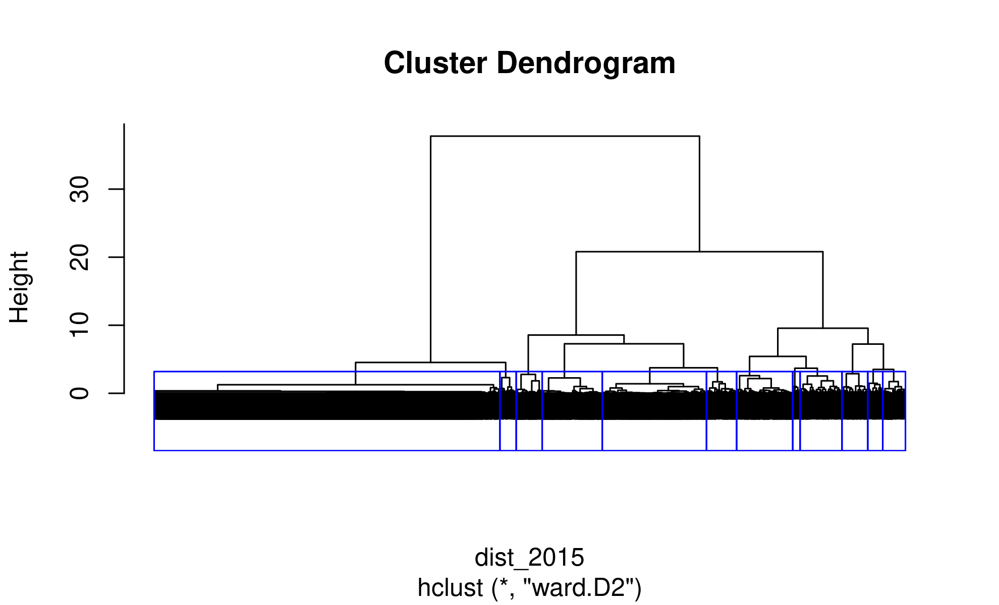
Finally, we add identifiers of the new clusters to our spatial object containing a grid of motifels and visualize it:

A map of Australia divided into twelve clusters based on the similarity of land cover composition

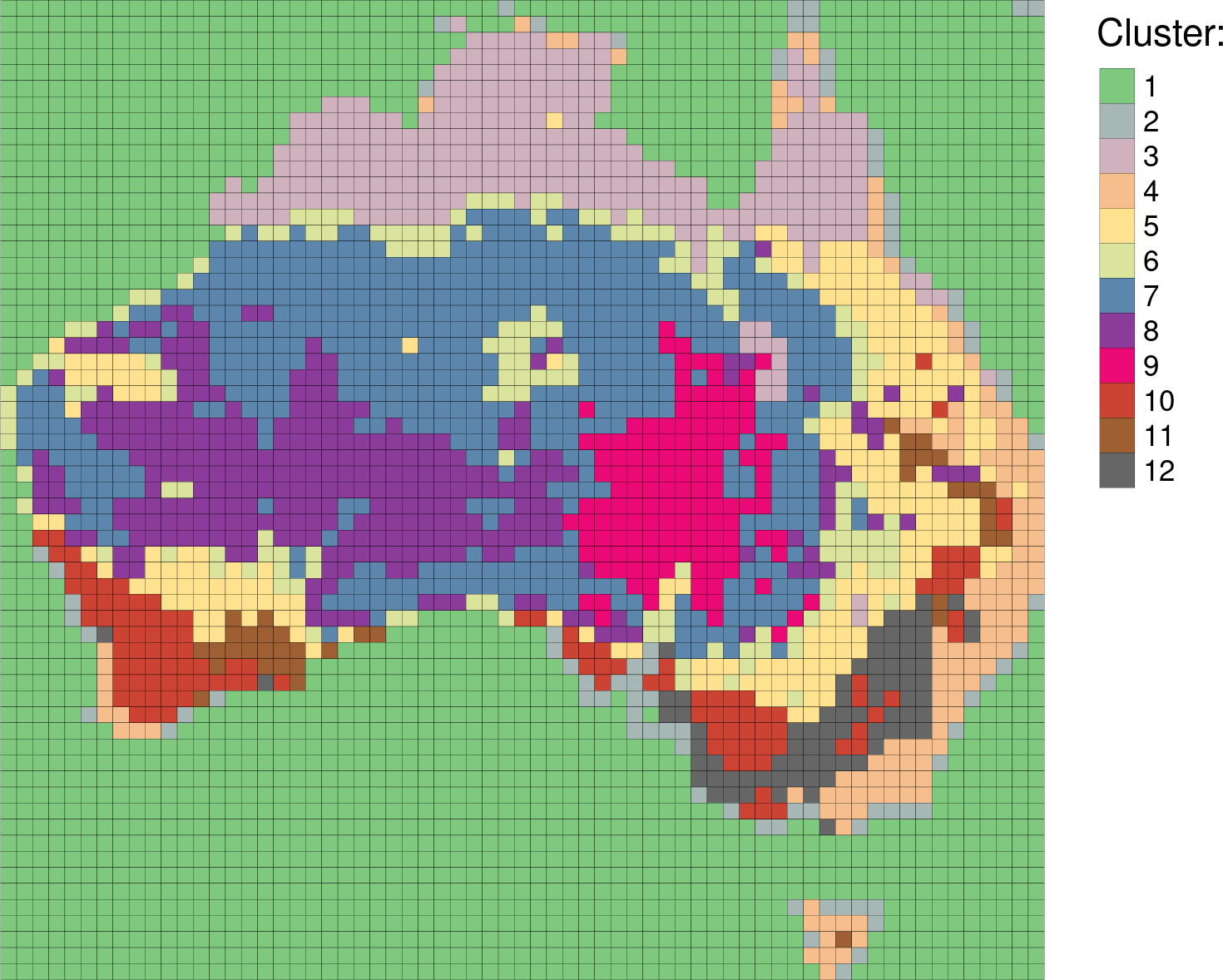
The output is a map with motifels grouped into the areas of the similar land cover composition. Some of the clusters represent one dominant land cover category, e.g. cluster 1 is water, cluster 3 is shrubland, and cluster 7 is sparse vegetation. On the other hand, some of the clusters can consist of many land cover categories. For example, cluster 6 is a mosaic of grassland and sparse vegetation and cluster 8 is a mosaic of sparse vegetation and shrubland.

Spatiotemporal pattern-based analysis

GeoPAT 2 also offers several additional features, including spatiotemporal pattern-based analysis. It is highly experimental, but already can be executed and tested. Let’s take a look at a couple examples from the GeoPAT 2 manual.

The input data is a set of twelve rasters of monthly sums of precipitation for the area of the British Isles from the WorldClim database. Each raster has 76560 pixels (240 rows and 319 columns). In other words, each pixel has 12 values representing temporal precipitation pattern.

Monthly sums of precipitation for the area of the British Isles

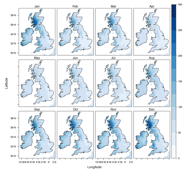
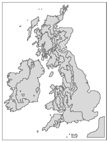
Many GeoPAT 2 methods for spatial data also work with spatiotemporal datasets. For example, it is possible to regionalize the British Isles based on its annual precipitation patterns. Each region has similar temporal precipitation pattern.

Regions of the similar annual precipitation patterns for the British Isles

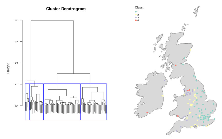
Another GeoPAT 2 application is clustering of spatiotemporal data. For example, we can extract temporal precipitation patterns of 97 largest cities in the British Isles and cluster them:

Example of a time series clustering

More information

Previous blog posts in the series introducing GeoPAT 2 - a software for pattern-based spatial and temporal analysis are:

1. GeoPAT 2: Software for Pattern-Based Spatial and Temporal Analysis
2. Pattern-based Spatial Analysis - core ideas
3. Finding similar local landscapes
4. Quantifying temporal change of landscape pattern
5. Pattern-based regionalization

If you want to learn more about the pattern-based spatial analysis read the official GeoPAT 2 manual. It contains installation instructions, description of the GeoPAT 2 architecture, several workflow paths with examples, and explanations of numerical signatures, dissimilarity measures, and topologies available in GeoPAT 2.

We also encourage users to submit issues and enhancement requests so we may continue to improve our software. Furthermore, if you have any question related to GeoPAT 2 please email me at nowosad.jakub@gmail.com.