
Blog posts in the series introducing GeoPAT 2 - a software for pattern-based spatial and temporal analysis:
- GeoPAT 2: Software for Pattern-Based Spatial and Temporal Analysis
- Pattern-based Spatial Analysis - core ideas
- Finding similar local landscapes
- Quantifying temporal change of landscape pattern
- Pattern-based regionalization
- Moving beyond pattern-based analysis: Additional applications of GeoPAT 2
This is a fourth blog post in the series introducing GeoPAT 2 - a software for pattern-based spatial and temporal analysis. The previous one focused on finding local landscapes with similar patterns. I had shown a small location of interest located in Australia and found a set of areas with very similar spatial patterns to it. Here, I will apply the concepts of the pattern-based spatial analysis to quantify temporal change of pattern in a fixed spatial location.
Introduction
Imagine you have two values expressing the world population in 1950 (2.5 billion people) and 2012 (7.1 billion people). How would you compare the change in the world population? The easiest (and correct) approach is just to subtract the past value from the more recent one:
\[ 7.1 - 2.5 = 4.6 \]
We can conclude that the world population between 1950 and 2015 increased by 4.6 billion people.
Now, let’s move into a more spatial problem. Think about how you can compare two satellite images or raster maps. Usually, the process is the same as in the example above - values in the image B are subtracted by values in the corresponding cells in the image A. This can be used to determine how land cover changes. Two raster land cover maps are just analyzed pixel by pixel, e.g. this pixel did change from forest to agriculture and that pixel did not change as it is classified as forest on both maps. It a good approach when we are interested in, e.g. overall changes over an extended area. This way you can say, for example, that globally in the last 25 year we lost this area of forest, but gain this area of agriculture.
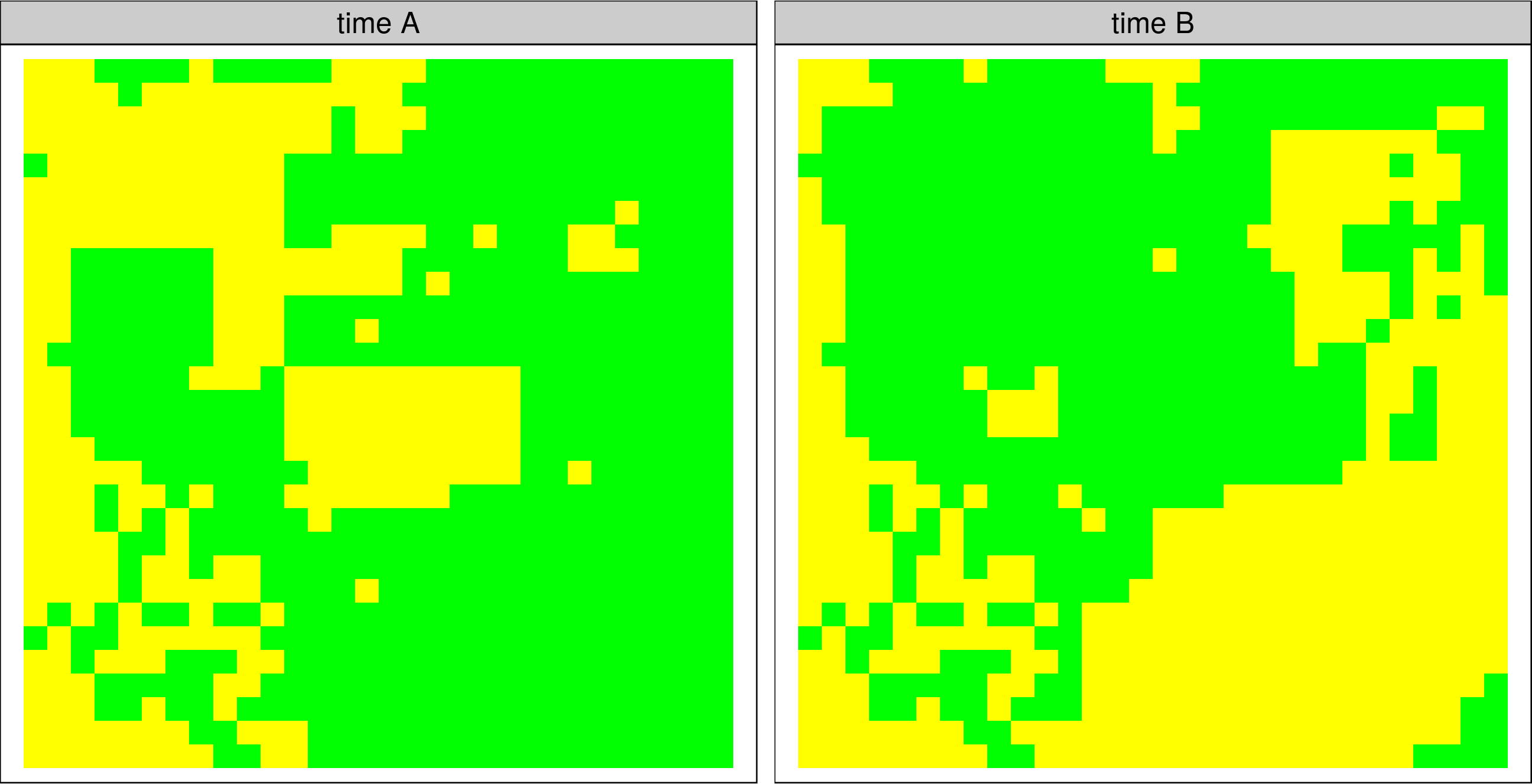
However, while this approach is helpful in many cases, it cannot solve all of the problems. Let’s consider these two areas, the left one represents an earlier time A and the right one represents a later time B.
When we compare it using the standard method (pixel by pixel) we get the result below:
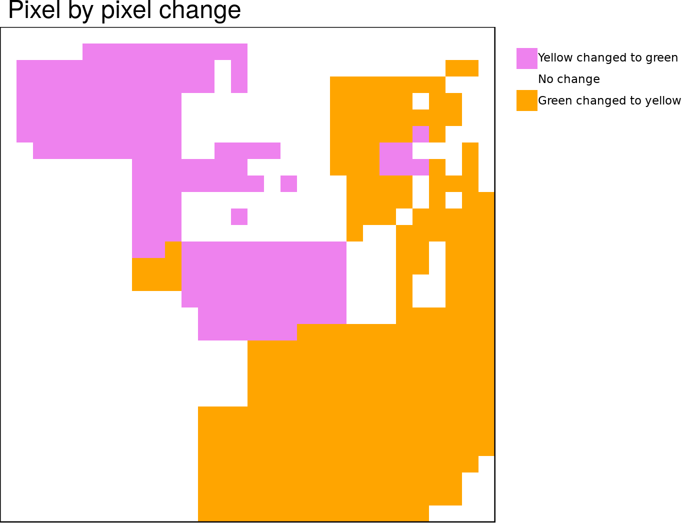
The changes analyzed this way are very prominent - about a half of the area had changed the category. However, when you look back at the whole landscape in time A and B, you should notice that both images are very similar if one disregards details and orientations. They both have the same number of categories, their share in the landscape is comparable and they are arranged in a similar spatial pattern. While we can say that many pixels have changed their values, we cannot say that this landscape’s pattern changed a lot. Therefore, to be able to fully describe the change of a landscape, we need to be able not only to see the changes in single pixels but also changes in spatial patterns.
Pixel by pixel analyses are a part of standard raster calculators, but comparing spatial patterns is a role for GeoPAT 2. This consists of two steps:
- Creating a grid of motifels.
- Comparing a query and a grid of motifels.
As an example, we are going to use land cover data of Australia from the year 2000 and 2015. To follow the subsequent calculations, you need to download both datasets, cci_lc2000.tif and cci_lc2015.tif, and install GeoPAT 2.
Creating grids of motifels
In the first step, we need to create two grids of motifels - one for each input raster.
{bash, eval = FALSE} gpat_gridhis -i cci_lc2000.tif -o patterns2000.grd -z 50 -f 50 -s cooc gpat_gridhis -i cci_lc2015.tif -o patterns2015.grd -z 50 -f 50 -s cooc
These grids, patterns2000.grd and patterns2015.grd, contain a large number of motifels that are represented by signatures. In the code above, we specify the input (-i) and the outputs (-o) files, while other parameters control a size of motifels and a signature used. Here, each motifel is a rectangle of 15,000 by 15,000 meters (-z 50: 50 pixels x map resolution of 300 meters). Importantly, motifels should not overlap, therefore we shift the subsequent motifels by 15,000 meters (-f 50: 50 pixels x map resolution of 300 meters). The last argument, -s, is crucial here. We can use -s prod that only represents shares of land cover categories or -s cooc, a spatial co-occurrence, that represents a spatial pattern.
Compare two maps
The second and final step is to use the outputs of the first step and compare their signatures. Three parameters are required here:
-i- this parameter is used twice, for the first and the second input grid (results of the first step)-o- a name of the output GeoTIFF file-m- selected similarity metric
{bash, eval = FALSE} gpat_compare -i patterns2000.grd -i patterns2015.grd -o similarity0015.tif -m jsd
The result is a raster map of similarities between Australia’s land cover in 2000 and 2015. Each pixel in this raster has a resolution of 15,000 meters and a value between 0 and 1. The largest value, 1, means that the spatial pattern in these two years is identical (no change in pattern has occured), while lower values represent areas with more and more dissimilar patterns (increasing degree of change in pattern has occured).
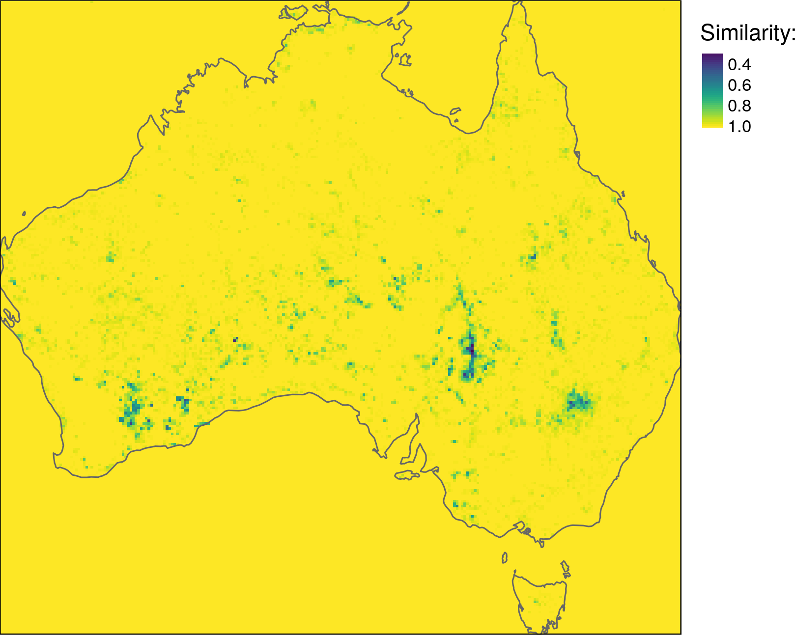
Large areas in northern and south-eastern Australia showed no change or very small change of spatial patterns of land cover (values of similarity close to 1). At the same time, there are a visible number of changed landscapes and their spatial distribution is not random. Now, they can be analyzed in more detail - we can look at what kind of landscapes changed the most (e.g. mosaic of forest and grassland), what is a trend in patterns changes (replacing grasslands with croplands), or what is the degree of spatial pattern changes.
Just to give you an example, below are six pairs of landscapes of different levels of similarity:
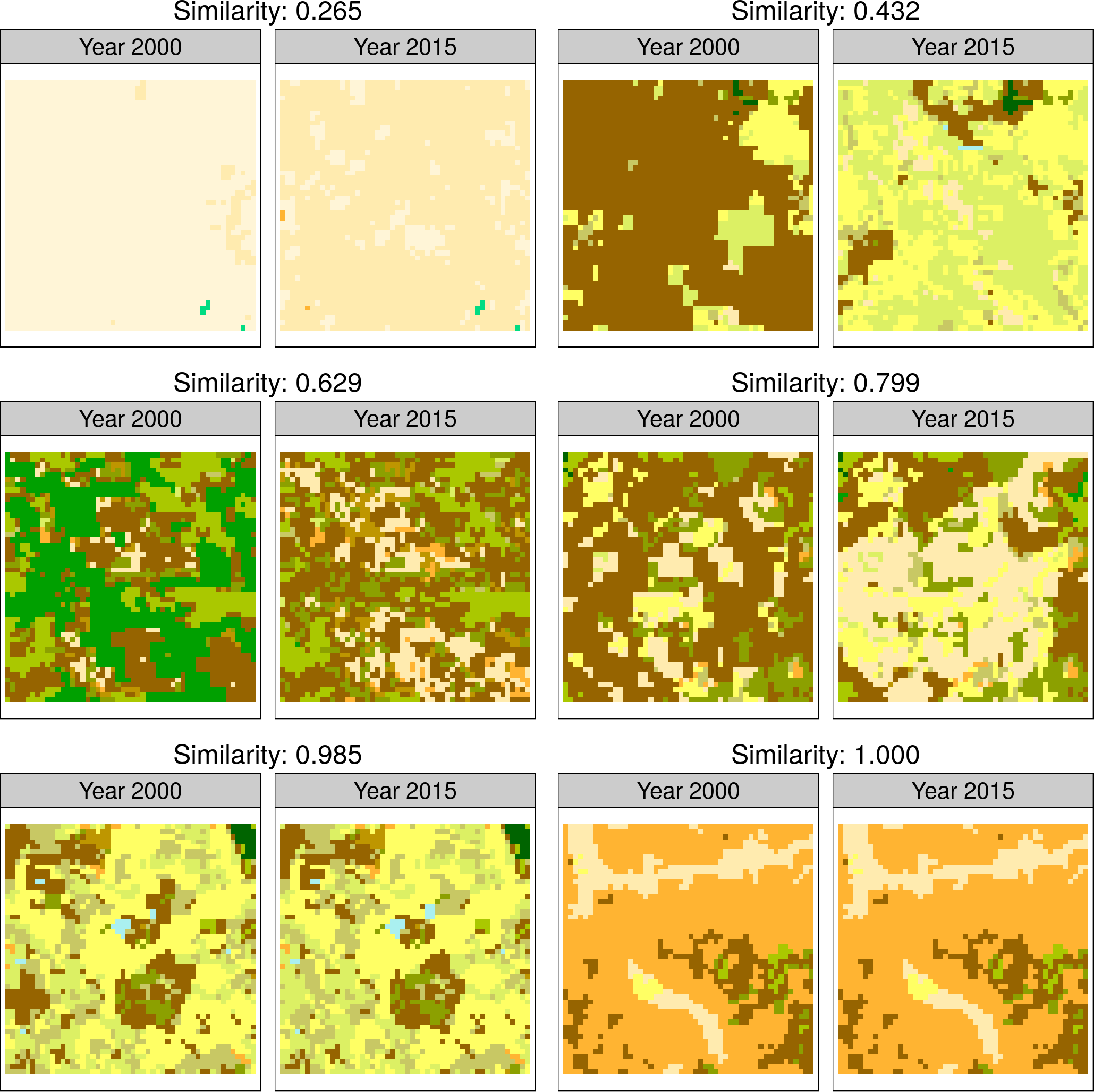
The most extreme example in top right corner represents an almost complete change from a bare area into a sparse vegetation. The next ones show decreasing levels of change, with the fifth example where just a small percentage of the area actually had changed. Finally, the last example has a similarity of 1, which means that its spatial pattern did not change.
What’s next
The next blog post in the GeoPAT 2 series is going to focus on automatic map regionalizations. In the meantime, you can find another simple example in the GeoPAT 2 user’s manual and if you want to see spatial pattern comparison in action, read a paper “Global mapping of changes in landscapes and coverages of vegetation types from the ESA land cover 1992-2015 time series”. It applies the pattern-based spatial analysis to describe global land cover changes during the 1992–2015 period.
Reuse
Citation
@online{nowosad2018,
  author = {Nowosad, Jakub},
  title = {Quantifying Temporal Change of Landscape Pattern},
  date = {2018-07-24},
  url = {https://jakubnowosad.com/posts/2018-07-24-geopat-2-compare/},
  langid = {en}
}