
Blog posts in the series introducing GeoPAT 2 - a software for pattern-based spatial and temporal analysis:
- GeoPAT 2: Software for Pattern-Based Spatial and Temporal Analysis
- Pattern-based Spatial Analysis - core ideas
- Finding similar local landscapes
- Quantifying temporal change of landscape pattern
- Pattern-based regionalization
- Moving beyond pattern-based analysis: Additional applications of GeoPAT 2
This is a fifth blog post in the series introducing GeoPAT 2 - a software for pattern-based spatial and temporal analysis. In the previous one we compared two raster images to quantify the temporal change of pattern in a fixed spatial location. Here, we focus on the most complex of the pattern-based analysis - segmentation. In other words, we will join areas of similar patterns in a way that they create homogeneous regions.
Introduction
Spatial patterns are an underexplored venue of the Earth and ecological sciences. They could be both an effect of some processes and at the same time affect other ones. For example, a land cover pattern (spatial arrangement of land cover categories) could exist because of an impact of a terrain topology, soils, climate, or human action. Next, this pattern can influence abiotic (e.g. some land cover patterns can be better to prevent erosion and flood than others) and biotic (e.g. some land cover patterns creates habitats for certain animals) components.
Although patterns are sometimes easy to see on a map, their delineation is difficult. Probably the most crucial obstacle is the undefinability of patterns’ borders. There is not a ground truth that enables you to validate which areas have a homogeneous pattern and where the line between two patterns should be drawn. Moreover, several practical problems exist - manual delineation of patterns is inconsistent, very often bias and hardly reproducible as different people have different definitions of patterns in their minds. On top of that there is an issue of time - how long would it take to create a detailed pattern-based regionalization on a global scale?
GeoPAT 2 provides a fast, consistent, but also a highly customizable way to regionalize space based on the underlining spatial patterns. It also has methods to analyze the quality of the output regionalization. The pattern-based segmentation process consists of three steps:
- Creating a grid of motifels.
- Regionalizing of homogeneous patterns.
- Obtaining quality of the segmentation.
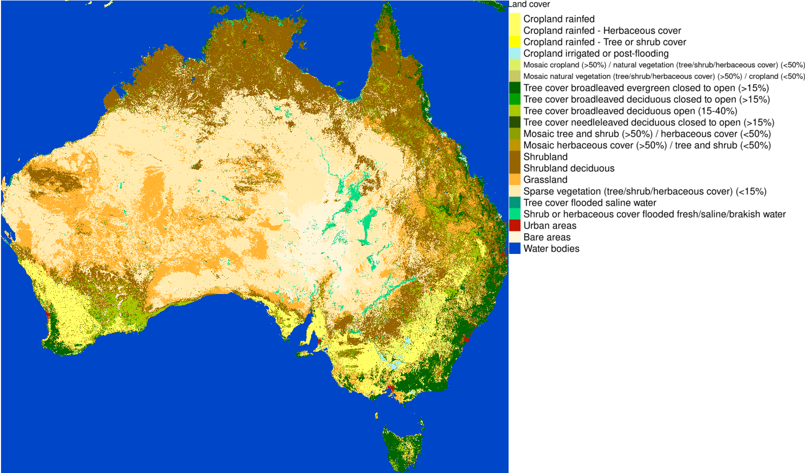
As an example, we are going to use land cover data of Australia from the year 2015. To follow the subsequent calculations, you need to download the dataset, cci_lc2015.tif, and install GeoPAT 2.
Creating grids of motifels
In the first step, we need to create a grid of motifels.
{bash, eval = FALSE} gpat_gridhis -i cci_lc2015.tif -o patterns2015.grd -z 25 -f 25 -s cooc
The patterns2015.grd grid contains a large number of motifels that are represented by the spatial coocurrence of categories. Motifels are rectangles of 7,500 by 7,500 meters (-z 25: 25 pixels x map resolution of 300 meters) covering the whole area of Australia. However, you need to keep in mind that they are going to be converted into “brick” blocks of 15,000 by 15,000 meters in the segmentation step. More about the “brick” topology in a moment…
Pattern-based segmentation
The second step is to create regions of homogeneous patterns using the output of the first step. Segmentation result depends on several parameters:
-i- an input grid of motifels (output from the first step)-o- a name of the output GeoTIFF file - the result in a raster format-v- a name of the output GeoPackage file - the result in a vector format-m- selected similarity metric--lthreshold- minimum distance threshold to build areas (see the examples below). It controls segments’ sizes--uthreshold- maximum distance threshold to build areas (see the examples below). It prevents the growth of inhomogeneous segments--swap- improve segmentation by swapping unmatched areas. 0 forces repetition until all unmatched segments will be swapped, while 1 skip this process--minarea- suppress creation of segments smaller than the set value--maxhist- decide how many neighbors are used to calculate similarity. When 0 is set it uses all of the neighbors, which can be time-consuming-q- set the root topology instead of the brick topology (see the examples below)-t- segmentation can be a computationally demanding process. This option allows using multiple CPU threads
Additional parameters are either experimental (--weights) or are used mostly for diagnostics purposes (-g, -r). Before digging deep into the parameters, let’s try and leave the default values of most of them:
{bash, eval = FALSE} # example A gpat_segment -i patterns2015.grd -o segments2015.tif -v segments2015.gpkg -m jsd -t 3
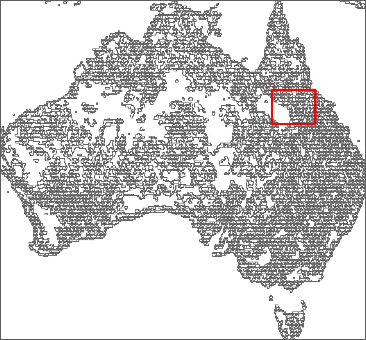
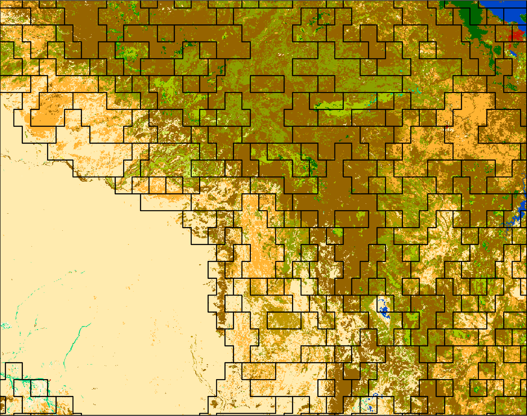
Using only three CPU threads, this process should take about four minutes on a modern laptop for the whole area of Australia. The result of the pattern-based segmentation consists of a large number of regions of varied size. Some of them are relatively small (one motifel) - they are different from the surrounding, while others span over large areas. To make it easier to see how segmentation works, let’s focus on the area in north-eastern Australia defined by the red rectangle:
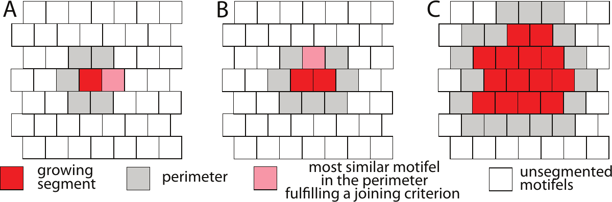
One of the most important concepts here is the way how motifels are created. Segmentation differs in this element from the rest of the spatial pattern-based analysis, as it uses so-called “brick topology”. Before the segmentation process can even start, grid created in the first step is transformed into a set “bricks” consisting of four motifels that are laid in alternate layers (see the figure below). Therefore, when you set the size to 25 in the first step, the segmented motifels would have a size of 50 by 50 cells (four motifels of 25 by 25). The “brick” topology allows creating segments using 6-connectivity, which gives better results than a simple 4-connectivity.
Segmentation process consists of several steps that are explained in the “Multi-scale segmentation algorithm for pattern-based partitioning of large categorical rasters” article. However, the most basic part to understand is how the segment growing works. We start from one motifel and calculate its similarity with all of the adjacent motifels. Next, we merge it with the most similar one and this process is repeated until we get to the threshold value:
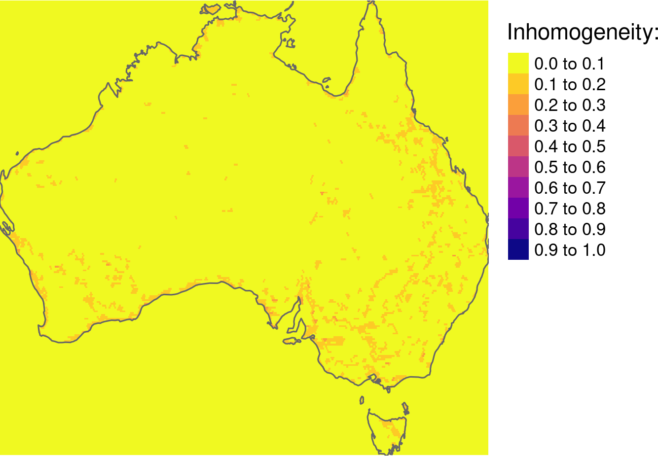
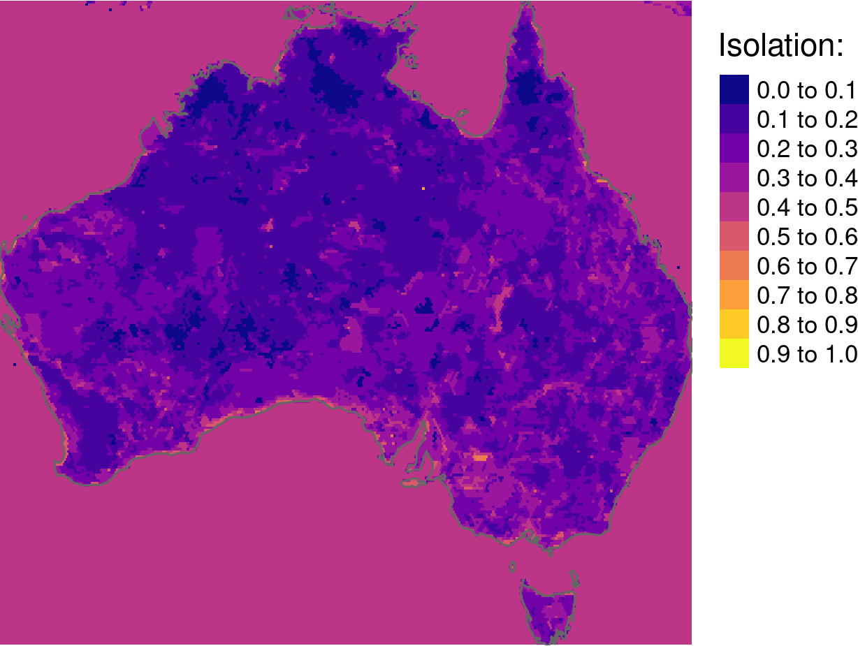
Segmentation quality
As I have mentioned in the introduction, ground truth does not exist in the pattern-based regionalization. However, we can measure several properties of the output segments and they could give us an insight into how good our results are.
{bash, eval = FALSE} gpat_segquality -i patterns2015.grd -s segments2015.tif -g inhomogeneity2015.tif -o isolation2015.tif
All of them have values between 0 and 1. The most important first-order property is inhomogeneity, which tells how internally inconsistent each segment is. Our main goal of segmentation is to obtain regions of homogeneous patterns, therefore we want this value to be as low as possible.
Secondary property of segmentation is isolation - we want regions that are distinct from their surroundings and therefore we aim for high values of isolation. However, you need to keep in mind that inhomogeneity and isolation are not equally important. You may want to obtain regions of homogeneous patterns that are not drastically isolated from surroundings, however isolated yet inhomogenous regions are usually meaningless.
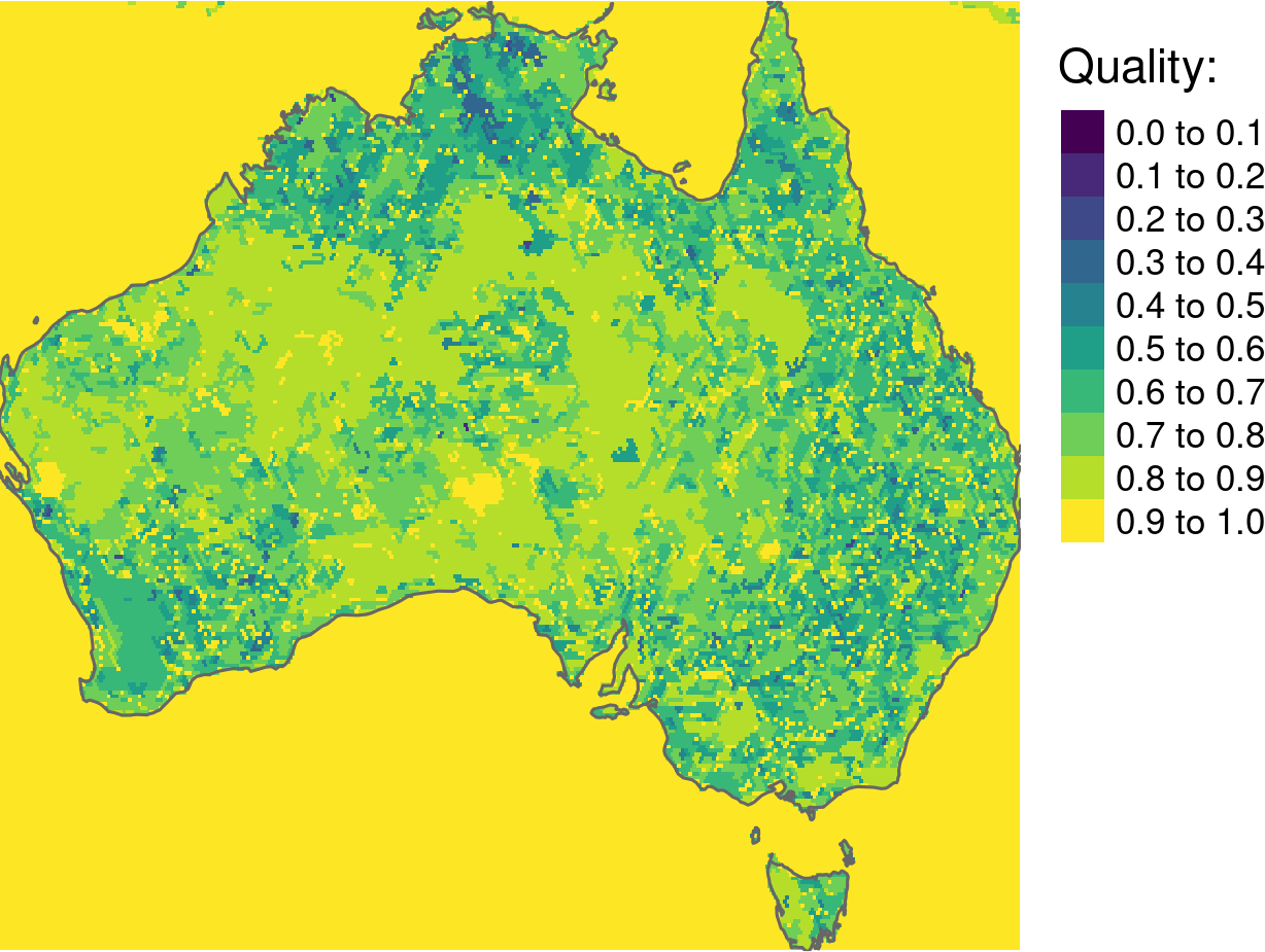
Finally, segmentation quality can be calculated as:
\[1 - (inhomogeneity/isolation)\]
It gives an overall metric of the output, where the larger the value the better.
Segmentation control
Pattern-based segmentation is a complex operation and visibly depends on several parameters mentioned above. Let’s try to manipulate some of them and see the results:
{bash, eval = FALSE} # example B gpat_segment -i patterns2015.grd -o segments2015_B.tif -v segments2015_B.gpkg -m jsd -t 3 --lthreshold=0.3 --uthreshold=0.5 # example C gpat_segment -i patterns2015.grd -o segments2015_C.tif -v segments2015_C.gpkg -m jsd -t 3 --minarea=6 # example D gpat_segment -i patterns2015.grd -o segments2015_D.tif -v segments2015_D.gpkg -m jac -t 3 # example E gpat_gridhis -i cci_lc2015.tif -o patterns2015_100.grd -s cooc -z 100 -f 100 gpat_segment -i patterns2015_100.grd -o segments2015_E.tif -v segments2015_E.gpkg -m jsd -t 3 -q
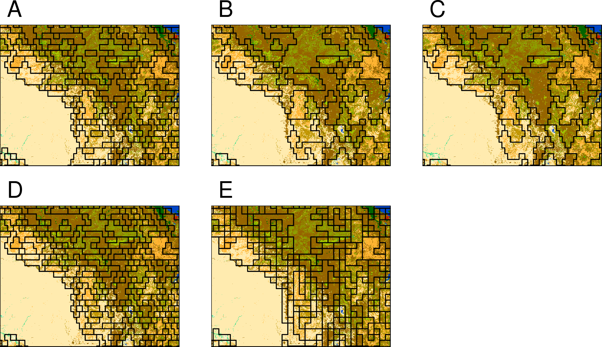
Example A uses the default values of the segmentation. In the second example (B), we increased values of two parameters, --lthreshold and --uthreshold. The first controls how homogenous the output regions should be in terms of patterns, with larger values indicating more inhomogenous regions (which also means larger regions/smaller number of segments). The second one prevents the growth of too large inhomogeneous segments. Example C has the --minarea parameter set to 6, which suppress creation of segments with fewer motifels than the set number. In example D, we used Jaccard distance, a different similarity measure. It gave fairly similar results to the Janson-Shannon divergence but different in details. And finally, example E used a root topology (also know as 4-connectivity). In the growing stage, it can only use neighbors from the left, right, top, and bottom. As a result, the output segmentation seems more clunky and the segments are aligned along horizontal and vertical lines.
What’s next
In the next blog post, I will show a few additional applications of GeoPAT 2 and how to adjust it to your own workflow. In the meantime, you can find other simple examples of segmentation as well as more detail explanation of the brick topology in the GeoPAT 2 user’s manual. If you are interested in a deeper explanation of the pattern-based segmentation, I encourage you to take a look at the article “Multi-scale segmentation algorithm for pattern-based partitioning of large categorical rasters”. It explains basic concepts (e.g. rook and brick topology), steps in the segmentation algorithm, and provides several examples. Finally, this method has been also applied for a machine ecoregionalization of terrestrial Earth’s landmass, where each ecophysiographic region was characterized by homogeneous physiography. You can read more about it at https://eartharxiv.org/fsver.
Reuse
Citation
@online{nowosad2018,
  author = {Nowosad, Jakub},
  title = {Pattern-Based Regionalization},
  date = {2018-08-13},
  url = {https://jakubnowosad.com/posts/2018-08-13-geopat-2-segmentation/},
  langid = {en}
}