How to calculate landscape metrics for local landscapes?

In the last few weeks, I was asked a similar question several times - how to calculate landscape metrics for local landscapes? In other words, how to divide the categorical input map into a number of smaller areas, and next calculate selected landscape metrics for each of the areas. Those areas have many names, such as tiles, squares, or motifels. The main goal of this post is to show how to calculate landscape metrics using the landscapemetrics R package.

To reproduce the results on your own computer, install and attach the following packages:

library(landscapemetrics)     # landscape metrics calculation
library(raster)               # spatial raster data reading and handling
library(sf)                   # spatial vector data reading and handling
library(dplyr)                # data manipulation

Reading the data

The first step is to read the input data.

data("augusta_nlcd")
my_raster = augusta_nlcd

In this example, we will use the augusta_nlcd dataset build in the landscapemetrics package. It is also possible to read any spatial raster file with the raster() function, for example my_raster = raster("path_to_my_file.tif"). The input file, however, should fulfill two requirements: (1) contain only integer values that represent categories, and (2) be in a projected coordinate reference system. You can check if your file meets the requirements using the check_landscape() function, and learn more about coordinate reference systems in the Geocomputation with R book.

Our example data looks like that:

plot(my_raster)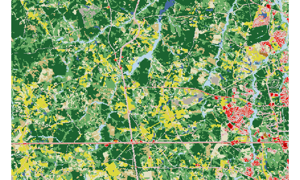

Creating a grid

One of the ways to create borders of local landscapes is to use the st_make_grid() function. This function accepts an sf object as the first argument, therefore we need to create a new object based on the bounding box of the input raster. Next, we also need to provide a second argument, either cellsize or n:

• cellsize - vector of length 1 or 2 - the side length of each grid cell in map units (usually meters)
• n - vector of length 1 or 2 - the number of grid cells in a row/column

my_grid_geom = st_make_grid(st_as_sfc(st_bbox(my_raster)), cellsize = 1500)
my_grid = st_sf(geom = my_grid_geom)

Next, we can overlay the newly created grid on top of our input raster:

plot(my_raster)
plot(my_grid, add = TRUE)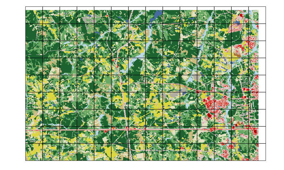

Calculating a metric

The calculation of landscape metrics for each cell can be done with the sample_lsm() function. It requires the input raster as the first argument, and the grid as the second one¹. Next, we can specify which landscape metrics we want to calculate. For example, we selected marginal entropy to be calculated on a landscape level. The complete list of the implemented metrics can be obtained with the list_lsm() function. Let us know if you are missing some metrics.

my_metric = sample_lsm(my_raster, my_grid,
                       level = "landscape", metric = "ent")
my_metric

## # A tibble: 126 x 8
##    layer level     class    id metric value plot_id percentage_inside
##    <int> <chr>     <int> <int> <chr>  <dbl>   <int>             <dbl>
##  1     1 landscape    NA    NA ent     2.54       1               100
##  2     1 landscape    NA    NA ent     2.52       2               100
##  3     1 landscape    NA    NA ent     2.47       3               100
##  4     1 landscape    NA    NA ent     2.49       4               100
##  5     1 landscape    NA    NA ent     2.38       5               100
##  6     1 landscape    NA    NA ent     2.48       6               100
##  7     1 landscape    NA    NA ent     2.65       7               100
##  8     1 landscape    NA    NA ent     2.41       8               100
##  9     1 landscape    NA    NA ent     2.28       9               100
## 10     1 landscape    NA    NA ent     2.44      10               100
## # … with 116 more rows

Each row in the my_metric object corresponds to each provided grid cell, with the values of marginal entropy in the value column ². Next, we can connect spatial grid with my_metric using the bind_cols() function:

my_grid = bind_cols(my_grid, my_metric)

The quickest visualization of the results can be done with the plot() function.

plot(my_grid["value"])

More complex vizualizations can be done with the tmap or ggplot2 packages.

Saving the results

The write_sf() function can save the results together with spatial geometry.

write_sf(my_grid, "my_grid.gpkg")

This output file can be read in any GIS software, such as QGIS, GRASS GIS, or ArcGIS.

Bonus 1 - show each raster

We can also see local landscapes for each grid cell, when we set the return_raster argument in sample_lsm() to TRUE:

my_metric_r = sample_lsm(my_raster, my_grid,
                         level = "landscape", metric = "ent",
                         return_raster = TRUE)
my_metric_r

## # A tibble: 126 x 9
##    layer level class    id metric value plot_id percentage_insi…
##    <int> <chr> <int> <int> <chr>  <dbl>   <int>            <dbl>
##  1     1 land…    NA    NA ent     2.54       1              100
##  2     1 land…    NA    NA ent     2.52       2              100
##  3     1 land…    NA    NA ent     2.47       3              100
##  4     1 land…    NA    NA ent     2.49       4              100
##  5     1 land…    NA    NA ent     2.38       5              100
##  6     1 land…    NA    NA ent     2.48       6              100
##  7     1 land…    NA    NA ent     2.65       7              100
##  8     1 land…    NA    NA ent     2.41       8              100
##  9     1 land…    NA    NA ent     2.28       9              100
## 10     1 land…    NA    NA ent     2.44      10              100
## # … with 116 more rows, and 1 more variable: raster_sample_plots <list>

This adds a new column, raster_sample_plots, that contains each local landscapes. Next, we can vizualize whichever landscapes we want, for example, number 1 which is located in the bottom left corner of the study area:

plot(my_metric_r$raster_sample_plots[[1]],
     main = paste0("ent: ", round(my_metric_r$value[[1]], 2)))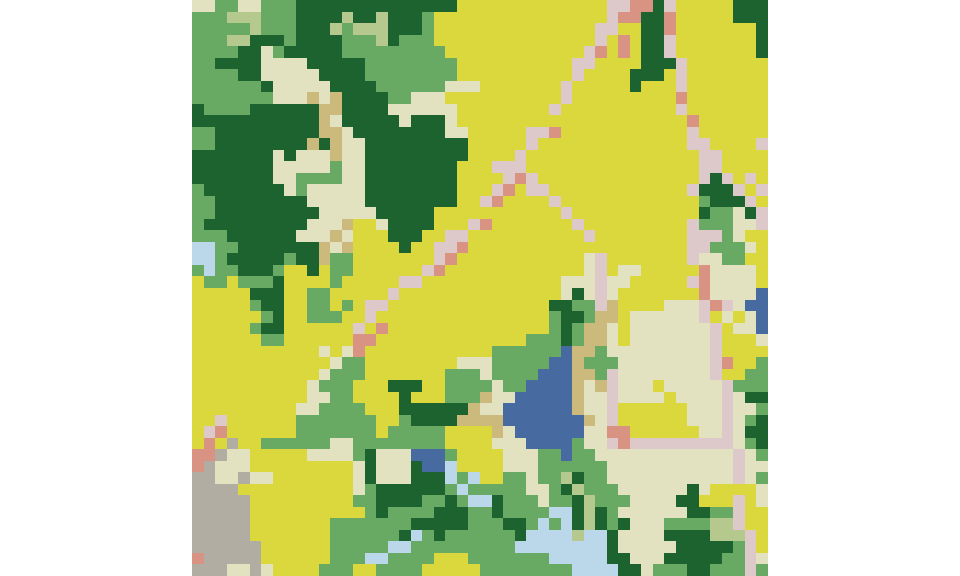

Bonus 2 - calculate many metrics

We are not limited to calculating just one metric at the time. The landscapemetrics package makes it possible to calculate up to 65 metrics on landscape level. There are several ways to specify the metrics we want to obtain as you can learn in the ?calculate_lsm help file. For this example, we selected two metrics - marginal entropy (abbriviation "ent") and mutual information (abbriviate as "mutinf"):

my_metrics = sample_lsm(my_raster, my_grid, 
                        level = "landscape", metric = c("ent", "mutinf"))
my_metrics

## # A tibble: 252 x 8
##    layer level     class    id metric value plot_id percentage_inside
##    <int> <chr>     <int> <int> <chr>  <dbl>   <int>             <dbl>
##  1     1 landscape    NA    NA ent    2.54        1               100
##  2     1 landscape    NA    NA mutinf 1.07        1               100
##  3     1 landscape    NA    NA ent    2.52        2               100
##  4     1 landscape    NA    NA mutinf 0.841       2               100
##  5     1 landscape    NA    NA ent    2.47        3               100
##  6     1 landscape    NA    NA mutinf 0.973       3               100
##  7     1 landscape    NA    NA ent    2.49        4               100
##  8     1 landscape    NA    NA mutinf 1.09        4               100
##  9     1 landscape    NA    NA ent    2.38        5               100
## 10     1 landscape    NA    NA mutinf 1.04        5               100
## # … with 242 more rows

The output data frame has two rows for each grid cell; therefore, if we want to connect the result with a spatial object, we need to reformat it. It can be done with the pivot_wider() function from the tidyr package.

library(tidyr)
my_metrics = pivot_wider(my_metrics, names_from = metric, values_from = value)
my_metrics

## # A tibble: 126 x 8
##    layer level     class    id plot_id percentage_inside   ent mutinf
##    <int> <chr>     <int> <int>   <int>             <dbl> <dbl>  <dbl>
##  1     1 landscape    NA    NA       1               100  2.54  1.07 
##  2     1 landscape    NA    NA       2               100  2.52  0.841
##  3     1 landscape    NA    NA       3               100  2.47  0.973
##  4     1 landscape    NA    NA       4               100  2.49  1.09 
##  5     1 landscape    NA    NA       5               100  2.38  1.04 
##  6     1 landscape    NA    NA       6               100  2.48  1.15 
##  7     1 landscape    NA    NA       7               100  2.65  1.12 
##  8     1 landscape    NA    NA       8               100  2.41  0.779
##  9     1 landscape    NA    NA       9               100  2.28  0.914
## 10     1 landscape    NA    NA      10               100  2.44  0.857
## # … with 116 more rows

This function moves metrics values from the value column into two new columns - ent and mutinf. Now, we are able to connect it to the spatial object with bind_cols():

my_grid2 = bind_cols(my_grid, my_metrics)

Plotting of the result requires providing the name of the column of a metric:

plot(my_grid2["ent"])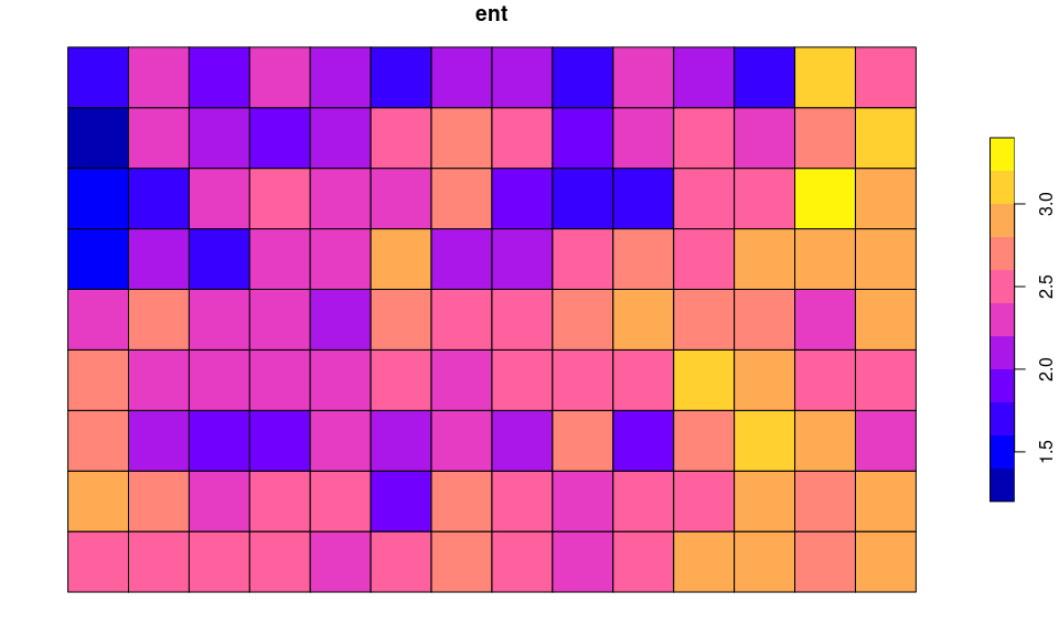

plot(my_grid2["mutinf"])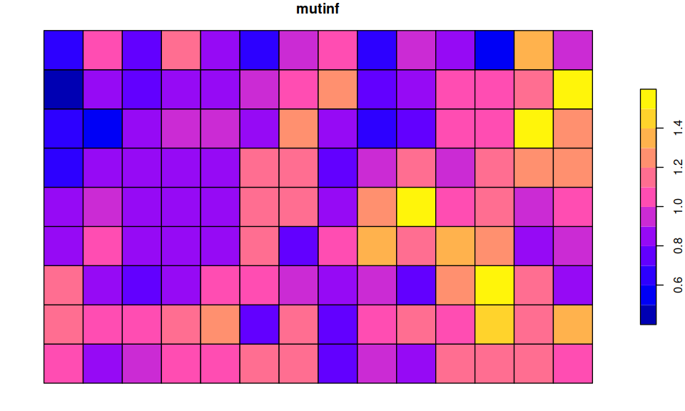

Summary

The sample_lsm() function offers more than calculations for regular areas. It is also possible to provide irregular polygons as the second argument and calculate any landscape metrics for them. The landscapemetrics package also has many additional features, including calculation of metrics in moving window with window_lsm() and in subsequential buffers around points of interest with scale_sample(). Learn more about landscape metrics and the landscapemetrics package at https://r-spatialecology.github.io/landscapemetrics/ and http://dx.doi.org/10.1111/ecog.04617.

Footnotes

1. This function also allows for many more possibilities, including specifying 2-column matrix with coordinates, SpatialPoints, SpatialLines, SpatialPolygons, sf points or sf polygons as the second argument. You can learn all of the possible options using ?sample_lsm.

2. To learn more about the structure of the output read the Efficient landscape metrics calculations for buffers around sampling points blog post.