Spatial patterns’ clustering
Jakub Nowosad
2025-07-26
Source:vignettes/articles/v5_cluster.Rmd
v5_cluster.RmdThe pattern-based spatial analysis makes it possible to find clusters of areas with similar spatial patterns. This vignette shows how to do spatial patterns’ clustering on example datasets. Let’s start by attaching necessary packages:
library(motif)
library(stars)
#> Loading required package: abind
#> Loading required package: sf
#> Linking to GEOS 3.13.0, GDAL 3.8.5, PROJ 9.5.1; sf_use_s2() is TRUE
library(sf)
safe_pal6 = c("#88CCEE", "#CC6677", "#DDCC77",
             "#117733", "#332288", "#888888")
safe_pal4 = c("#88CCEE", "#CC6677", "#DDCC77", "#117733")
Spatial patterns’ clustering requires one spatial object. For this
vignette, we will read the "raster/landcover2015.tif"
file.
landcover = read_stars(system.file("raster/landcover2015.tif", package = "motif"))This file contains a land cover data for New Guinea, with seven possible categories: (1) agriculture, (2) forest, (3) grassland, (5) settlement, (6) shrubland, (7) sparse vegetation, and (9) water.
landcover = droplevels(landcover)
plot(landcover, key.pos = 4, key.width = lcm(5), main = NULL)
#> downsample set to 12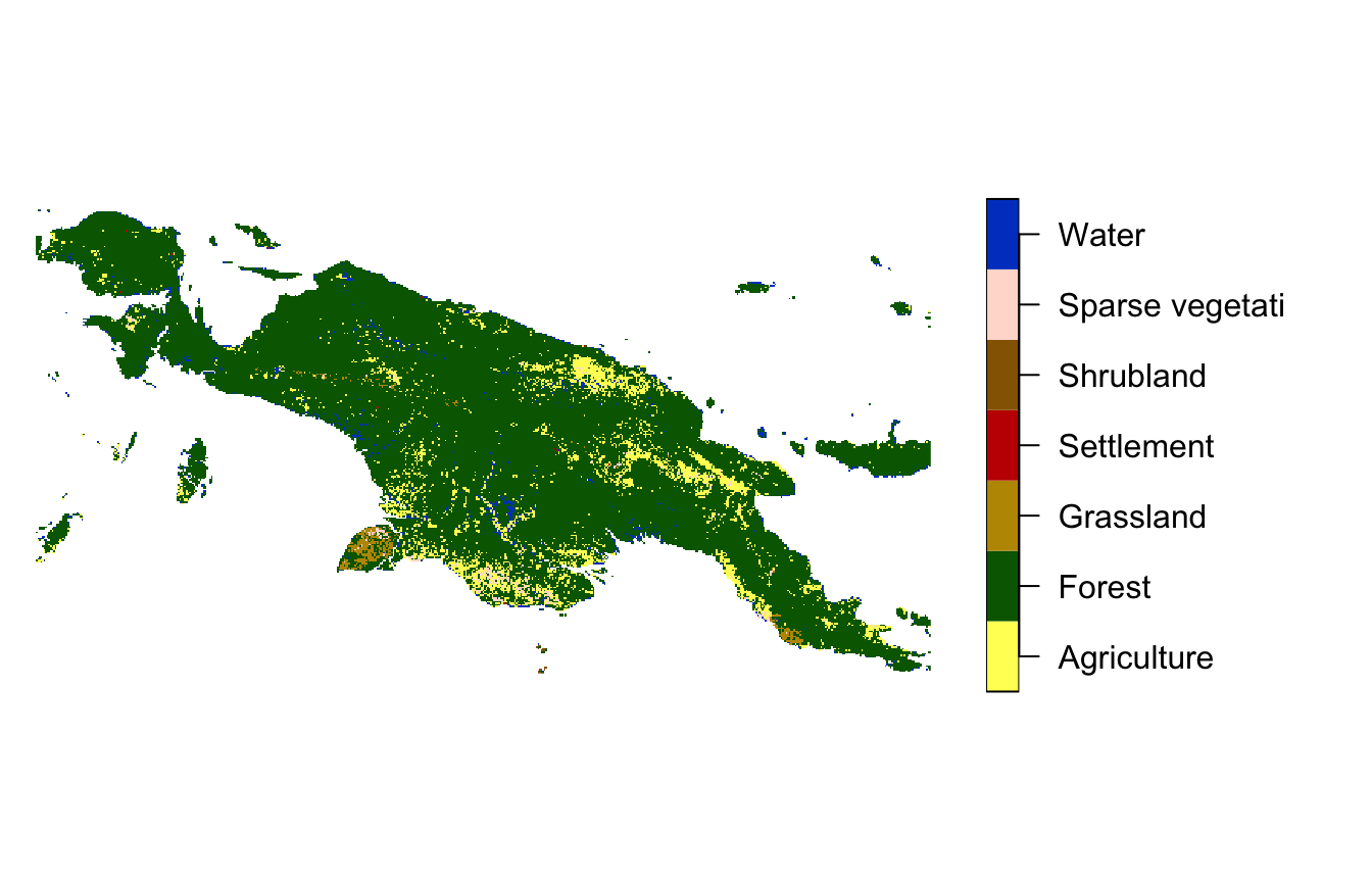
Regular local landscapes
In the first example, we divide the whole area into many regular local landscapes, and find a way to cluster them based on their patterns.
#> downsample set to 12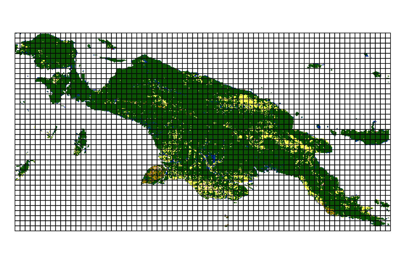
It starts with calculating a signature for each local landscape using
the lsp_signature() function. Here, we use the
co-occurrence vector (type = "cove") representation on
local landscapes of 100 by 100 cells (window = 100).
Distance measures, used in one of the next steps, often require
normalization of the vector, therefore we transform the representation
to sum to one.
landcover_cove = lsp_signature(landcover, type = "cove",
                                window = 100, normalization = "pdf")
Read the Introduction to the motif package vignette to learn more about spatial signatures.
Next, we need to calculate the distance (dissimilairy) between each
local landscape’s pattern. This can be done with the
lsp_to_dist() function, where we must provide the output of
lsp_signature() and a distance/dissimilarity measure used
(dist_fun = "jensen-shannon").
landcover_dist = lsp_to_dist(landcover_cove, dist_fun = "jensen-shannon")
#> Metric: 'jensen-shannon' using unit: 'log2'; comparing: 1080 vectors.
The output, landcover_dist, is of a dist
class.
class(landcover_dist)
#> [1] "dist"
This allows it to be used by many existing R functions for
clustering, which expect a distance matrix (dist) as an
input. It includes different approaches of hierarchical clustering
(hclust(), cluster::agnes(),
cluster::diana()) or fuzzy clustering
(cluster::fanny()). More information about clustering
techniques in R can be found in CRAN Task View:
Cluster Analysis & Finite Mixture Models.
We use a hierarchical clustering using hclust() in this
example. It needs a distance matrix as the first argument and a linkage
method as the second one. Here, we use method = "ward.D2",
which means that we are be using Ward’s minimum variance method that
minimizes the total within-cluster variance.

Graphical representation of the hierarchical clustering is called a
dendrogram. Based on the obtained dendrogram, we can divide our local
landscapes into a specified number of groups using
cutree(). In this example, we use six classes
(k = 6) to make a result fairly straightforward to
understand.
clusters = cutree(landcover_hclust, k = 6)The motif package allows representing the clustering
results as either sf or stars object. This can
be done with the lsp_add_clusters() function.
sf
By the default, it creates a sf object with a new
variable clust:
landcover_grid_sf = lsp_add_clusters(landcover_cove, clusters)
plot(landcover_grid_sf["clust"], pal = safe_pal6)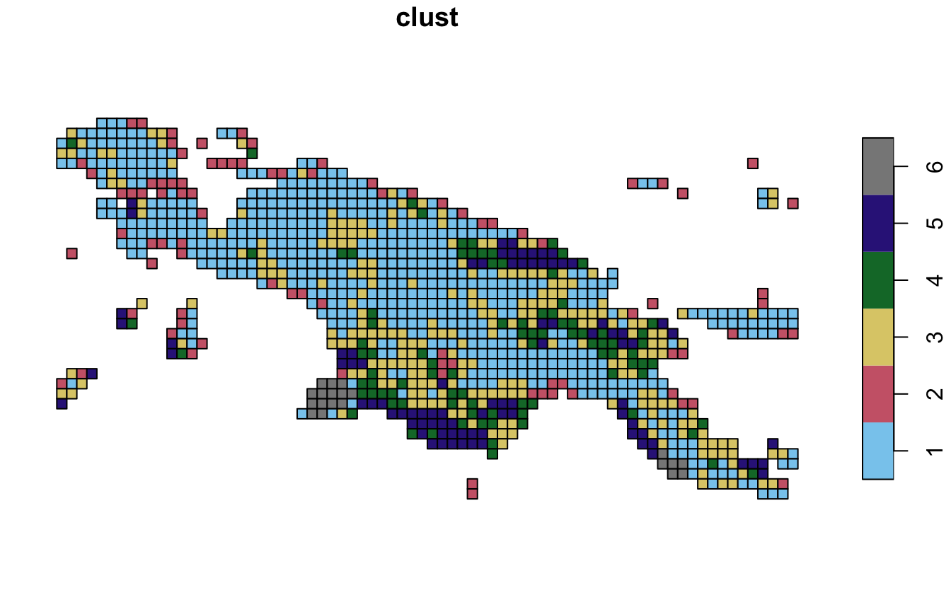
Samples
Now, it is possible see some examples of each cluster.
For example, we can get id values of randomly selected local landscapes from the first cluster.
landcover_grid_sf_1 = subset(landcover_grid_sf, clust == 1)
sample(landcover_grid_sf_1$id, 3)
#> [1] 1146 1070 1376
Next, we can extract them using lsp_extract(). This
cluster contains landscapes mostly covered by forest with small areas of
agriculture.
plot(lsp_extract(landcover, window = 100, id = 1229), key.pos = NULL)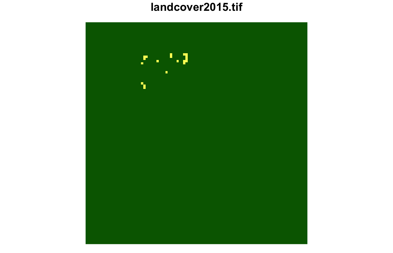
plot(lsp_extract(landcover, window = 100, id = 1237), key.pos = NULL)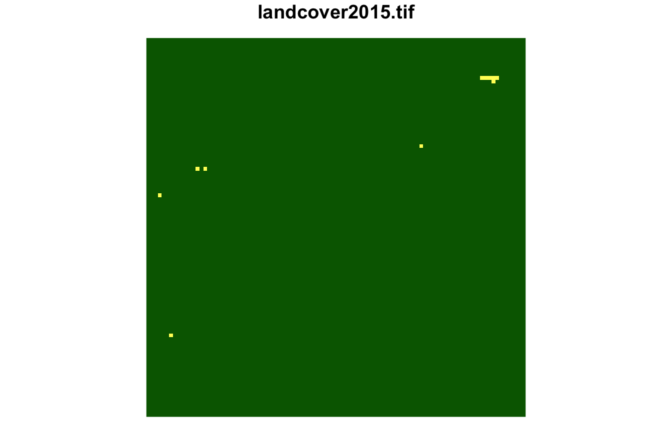
plot(lsp_extract(landcover, window = 100, id = 687), key.pos = NULL)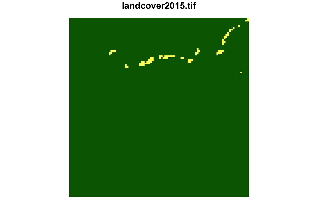
This approach can be used for any other cluster.
landcover_grid_sf_6 = subset(landcover_grid_sf, clust == 6)
sample(landcover_grid_sf_6$id, 3)
#> [1] 2579 2027 2577
The sixth cluster is covered by frest, grassland, with smaller areas of water and sparse vegetation.
plot(lsp_extract(landcover, window = 100, id = 2098), key.pos = NULL)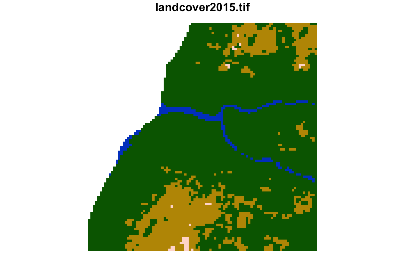
plot(lsp_extract(landcover, window = 100, id = 2173), key.pos = NULL)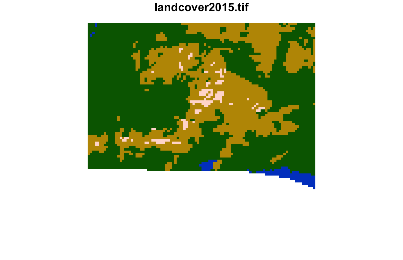
plot(lsp_extract(landcover, window = 100, id = 2172), key.pos = NULL)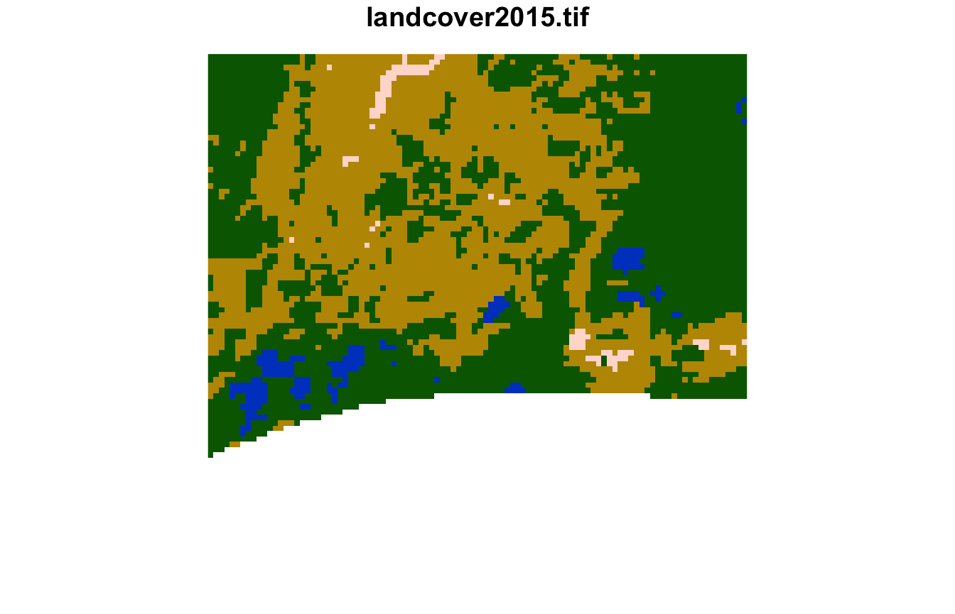
Quality
We can also calculate the quality of the clusterings with the
lsp_add_quality() function, which requires an output of
lsp_add_clusters() as the first argument and output of
lsp_to_dist() as the second one. It adds three new
variables: inhomogeneity, distinction, and
quality.
landcover_grid_sfq = lsp_add_quality(landcover_grid_sf, landcover_dist)Inhomogeneity (inhomogeneity) measures a degree of
mutual dissimilarity between all objects in a cluster. This value is
between 0 and 1, where the small value indicates that all objects in the
cluster represent consistent patterns so the cluster is
pattern-homogeneous.
inhomogeneity_pal = hcl.colors(6, palette = "Emrld")
plot(landcover_grid_sfq["inhomogeneity"], pal = inhomogeneity_pal)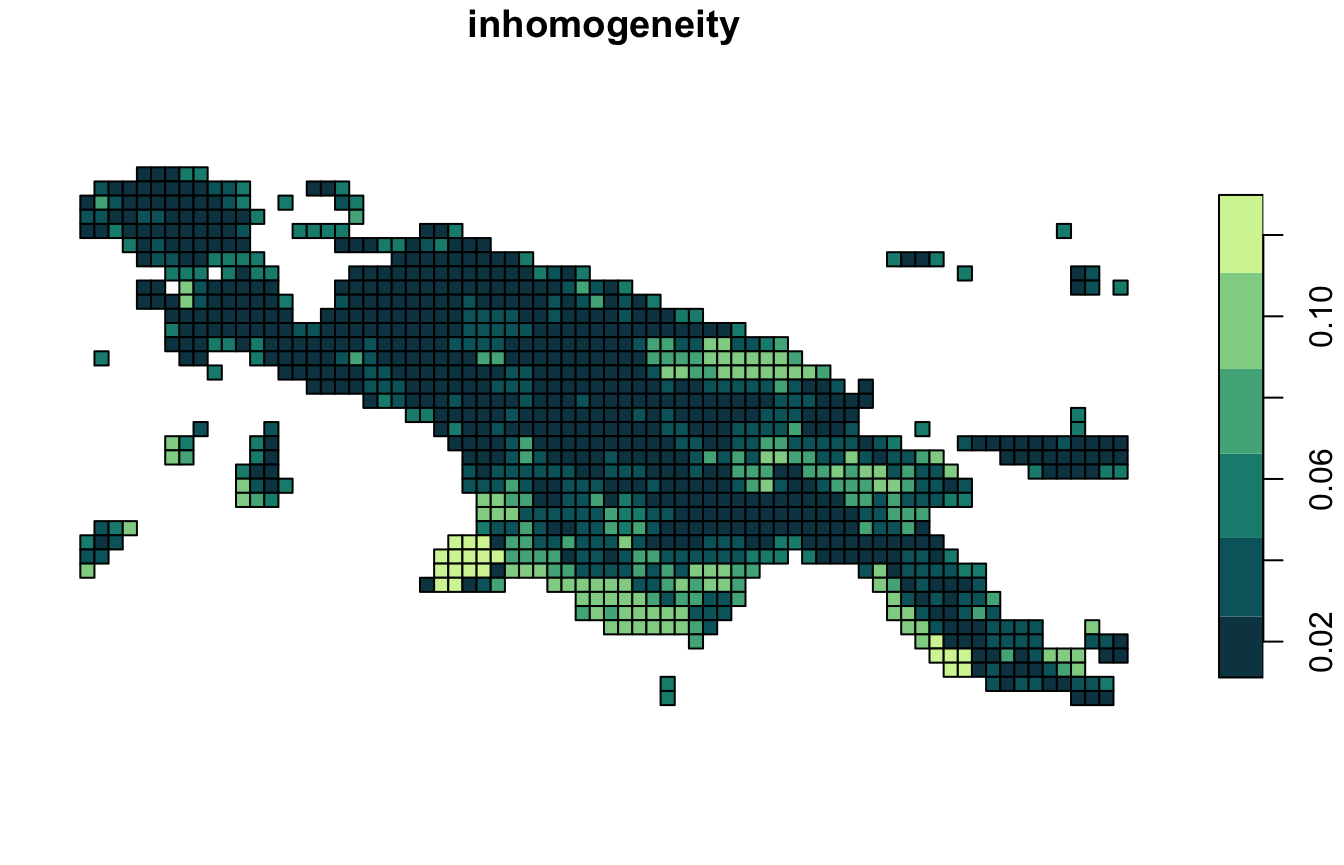
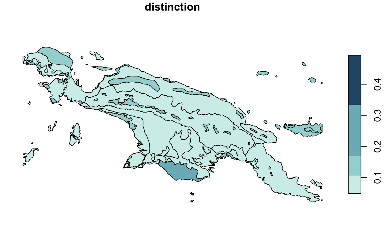
Distinction (distinction) is an average distance between
the focus cluster and all the other clusters. This value is between 0
and 1, where the large value indicates that the cluster stands out from
the rest of the clusters.
distinction_pal = hcl.colors(6, palette = "Teal", rev = TRUE)
plot(landcover_grid_sfq["distinction"], pal = distinction_pal)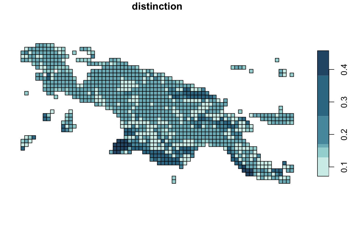
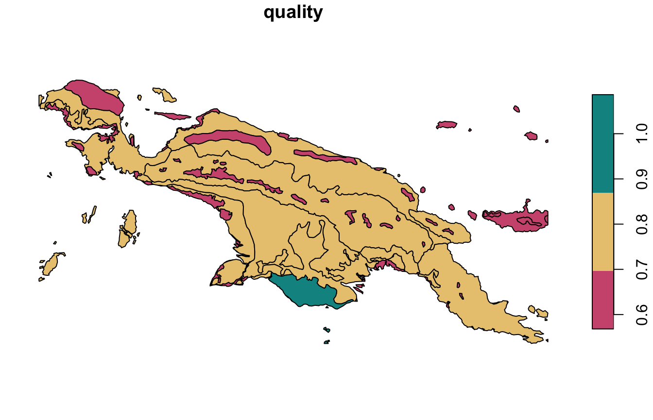
Overall quality (quality) is calculated as
1 - (inhomogeneity / distinction). This value is also
between 0 and 1, where increased values indicate increased quality of
clustering.
quality_pal = hcl.colors(6, palette = "Temps", rev = TRUE)
plot(landcover_grid_sfq["quality"], pal = quality_pal)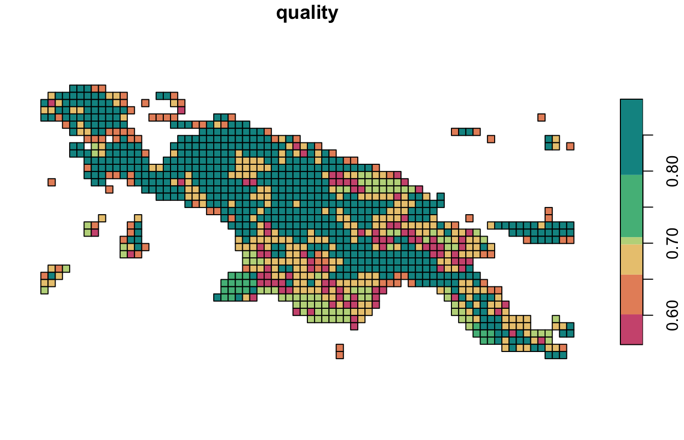
stars
To create an stars object with a new attribute
clust, we must set output = "stars".
landcover_grid_stars = lsp_add_clusters(landcover_cove, clusters, output = "stars")
plot(landcover_grid_stars["clust"], col = safe_pal6)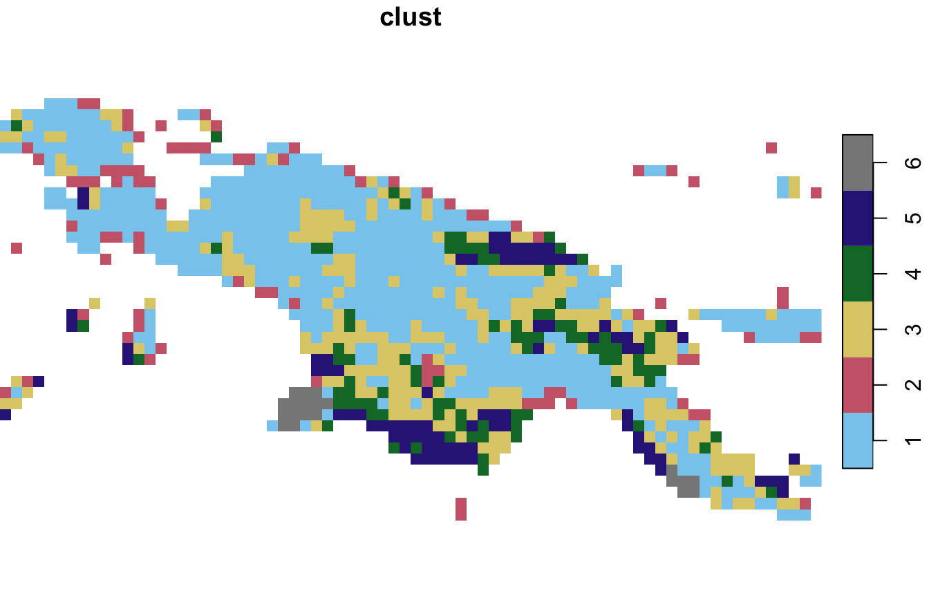
However, it is not yet possible to calculate the quality of the
clusterings for the stars objects:
landcover_grid_starsq = lsp_add_quality(landcover_grid_stars, landcover_dist)
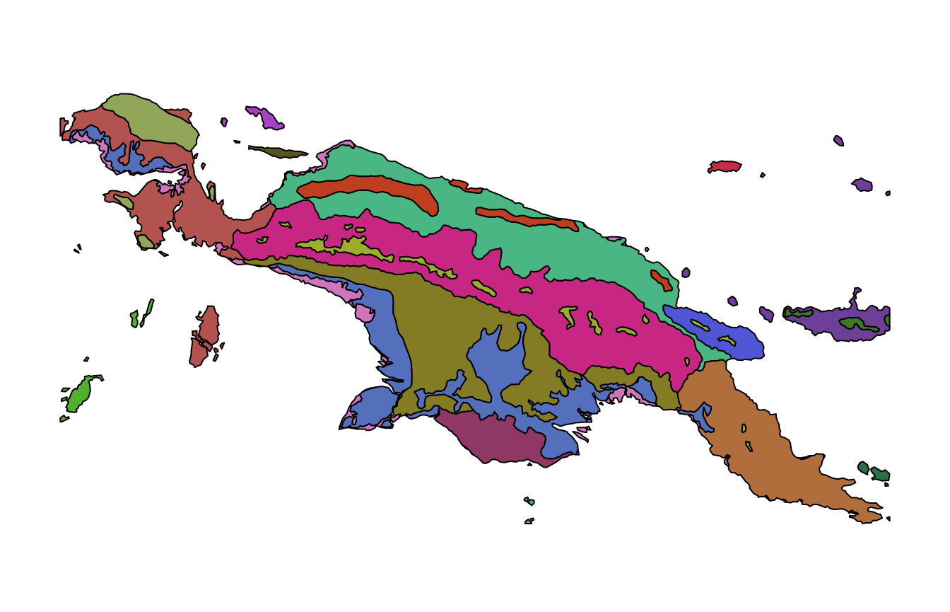
#> Error: This function requires an sf object as the x argument.Irregular local landscapes
The motif package also allows for the clustering of
irregular regions based on the user-provided polygons. It has an example
spatial vector dataset, ecoregions.gpkg, which contains
terrestrial ecoregions for New Guinea from https://ecoregions2017.appspot.com/.
ecoregions = read_sf(system.file("vector/ecoregions.gpkg", package = "motif"))This dataset has 22 rows, where each row relates to one ecoregion.
Each ecoregion is also related to a unique value in the id
column.
The first step here is to calculate a signature for each ecoregion
using lsp_signature():
landcover_cove2 = lsp_signature(landcover, type = "cove",
                                 window = ecoregions["id"], normalization = "pdf")
Next step involves calculating distances between signatures of ecoregions:
landcover_dist2 = lsp_to_dist(landcover_cove2, dist_fun = "jensen-shannon")
#> Metric: 'jensen-shannon' using unit: 'log2'; comparing: 22 vectors.
Again, we find clusters using a hierarchical clustering:

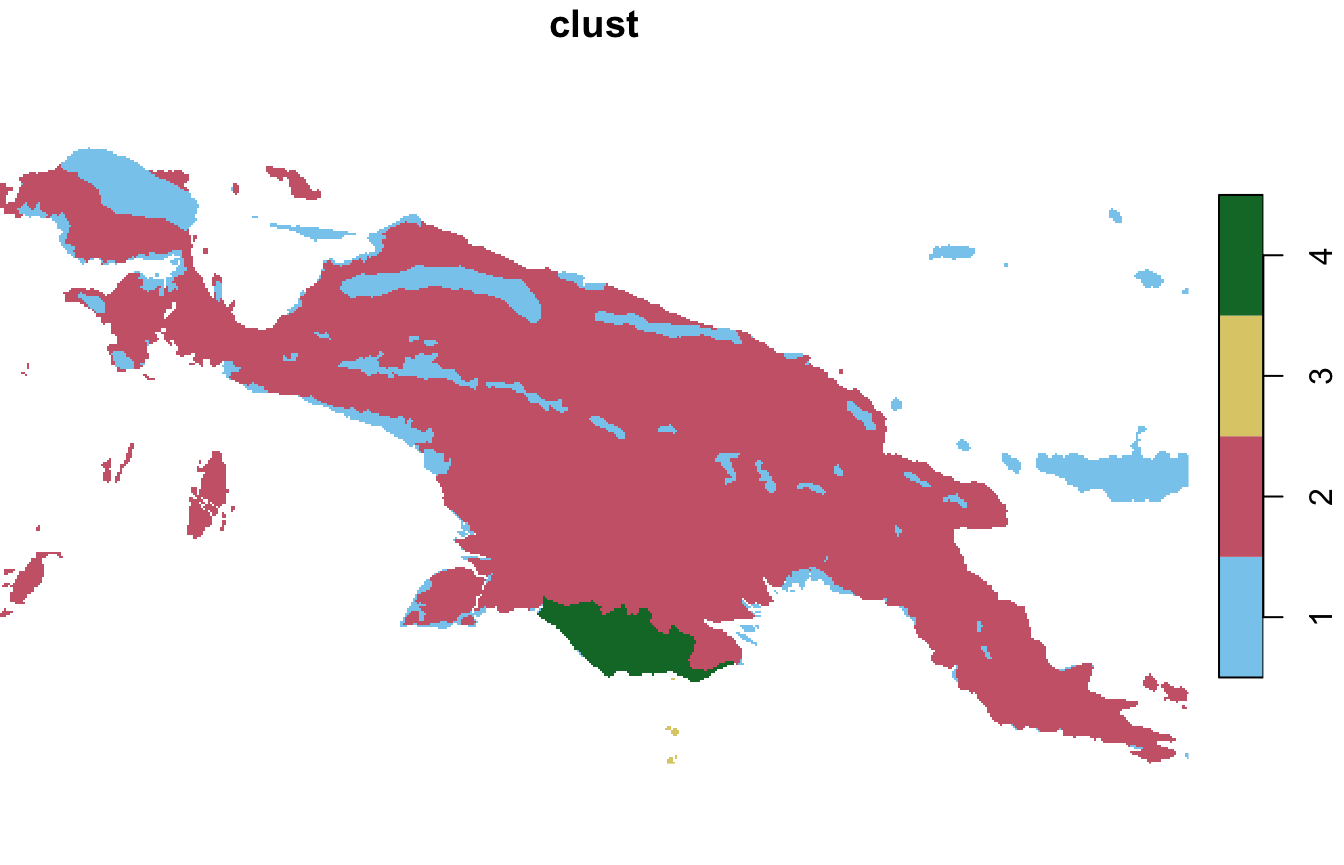
This time, we divide the data into four clusters:
clusters2 = cutree(landcover_hclust2, k = 4)
sf
Next steps are to add clusters ids to the sf object:
landcover_grid_sf2 = lsp_add_clusters(landcover_cove2, clusters2,
                                      window = ecoregions["id"])
The results show that most area of New Guinea belongs to the second clusters, with only one ecoregion of cluster 3 (small islands south from New Guinea) and cluster 4.
plot(landcover_grid_sf2["clust"], pal = safe_pal4)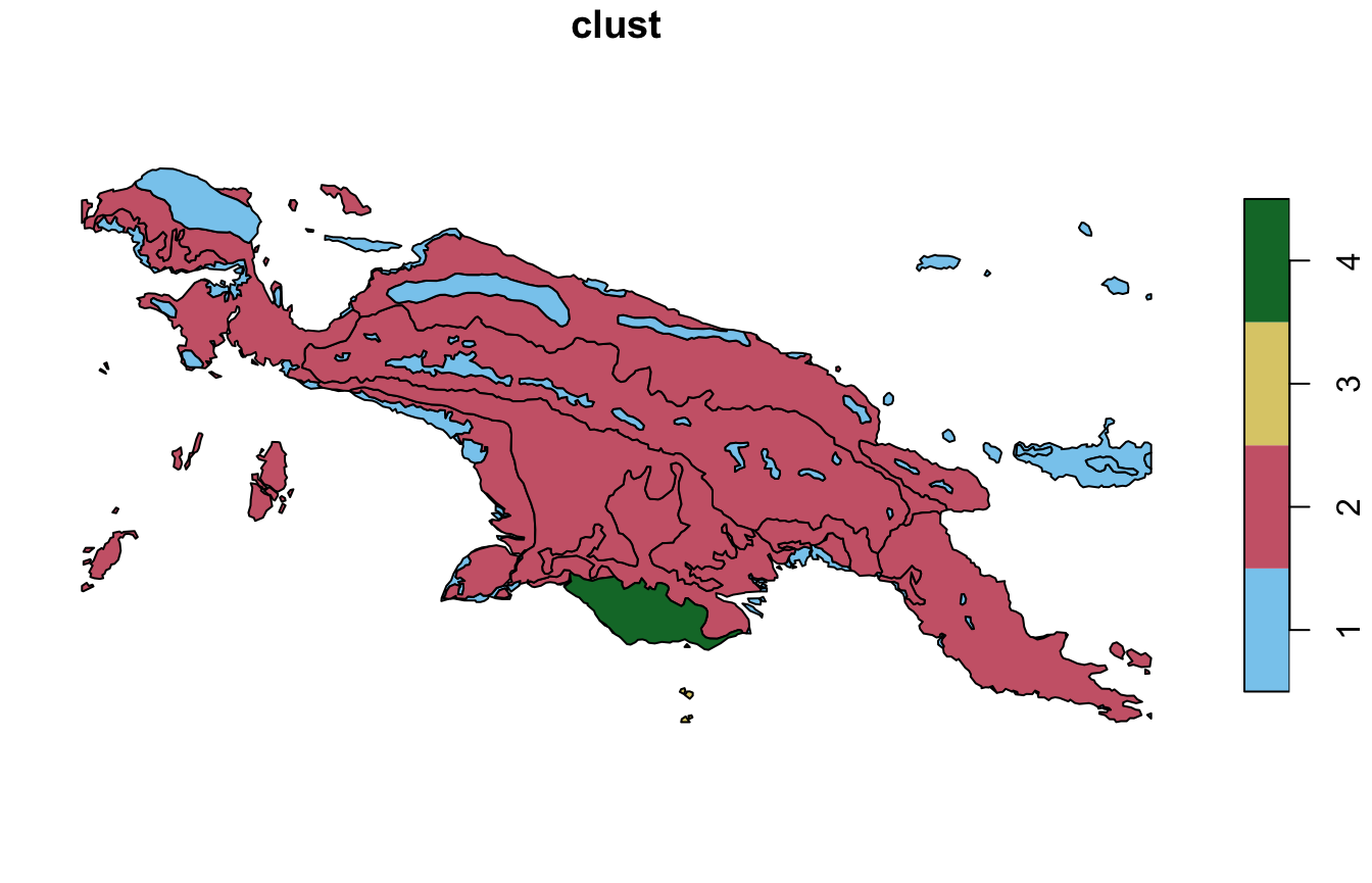
Samples
The first cluser, for example, consists of nine ecoregions, from which we sampled only three.
landcover_grid_sf2_1 = subset(landcover_grid_sf2, clust == 1)
sample(landcover_grid_sf2_1$id, 3)
#> [1] 10  1 22
Next, we can extract their land cover using
lsp_extract(). This cluster contains landscapes mostly
covered by forest with small areas of agriculture.
plot(lsp_extract(landcover, window = ecoregions["id"], id = 10), key.pos = NULL)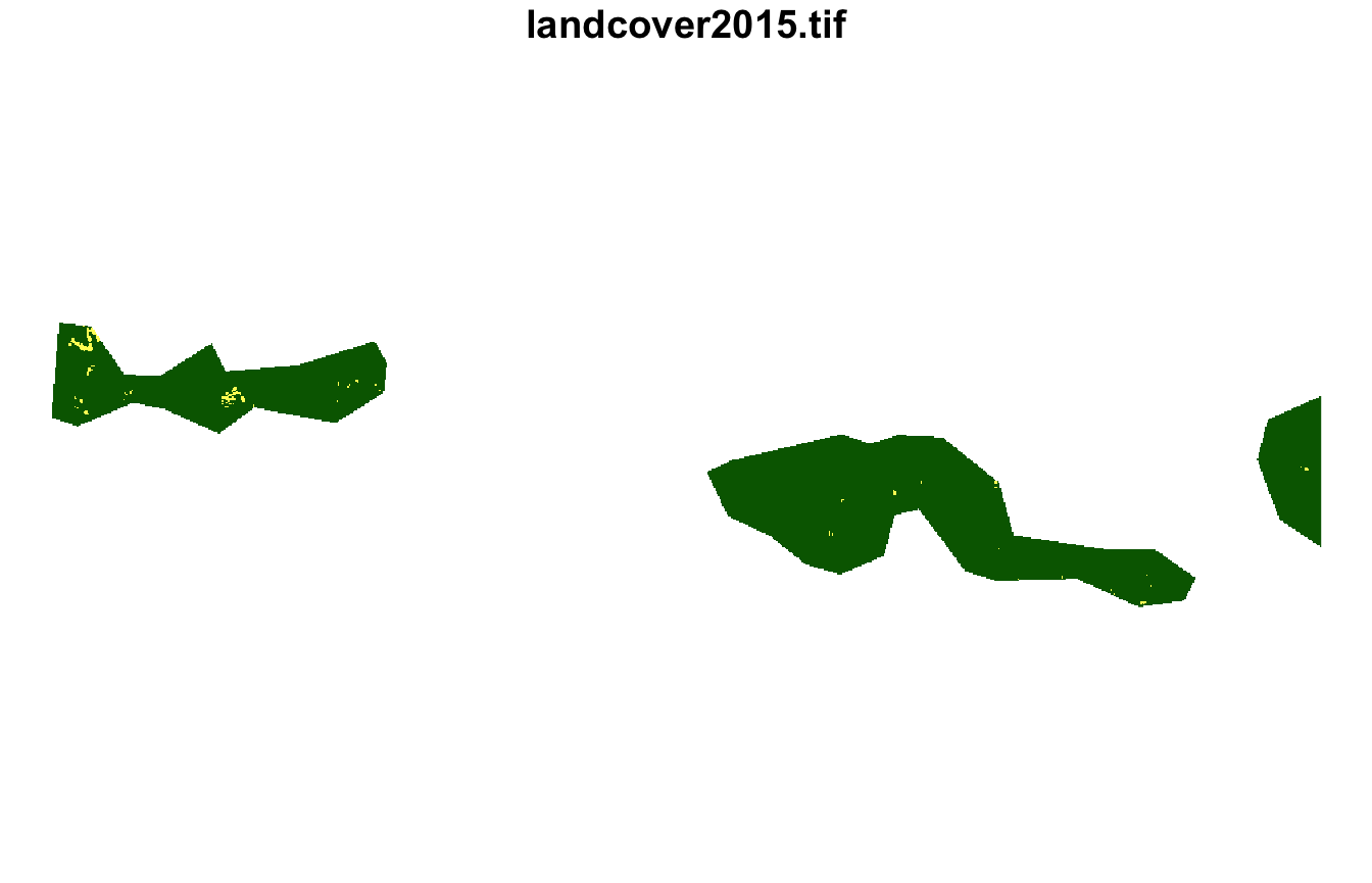
plot(lsp_extract(landcover, window = ecoregions["id"], id = 1), key.pos = NULL)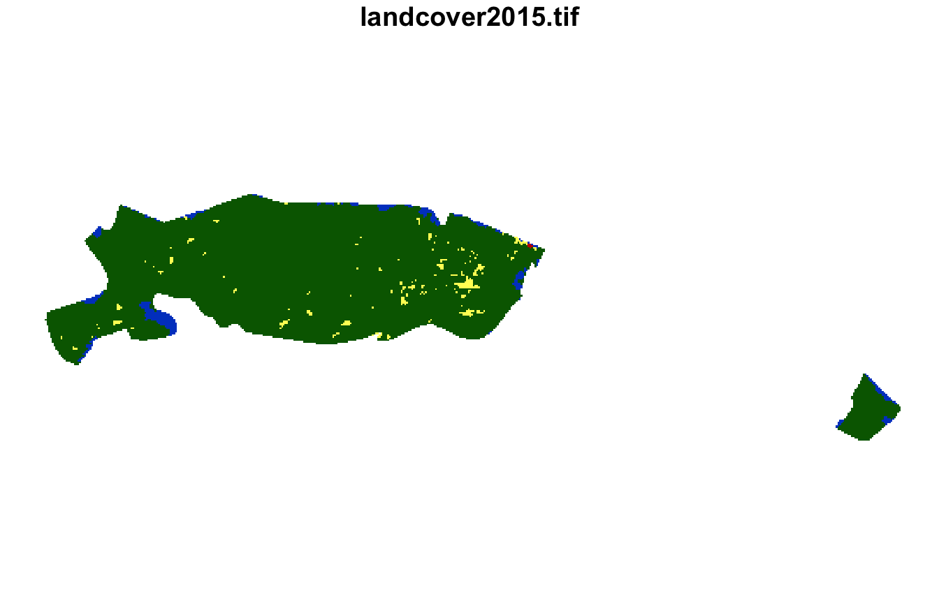
plot(lsp_extract(landcover, window = ecoregions["id"], id = 22), key.pos = NULL)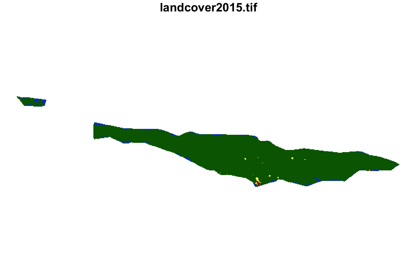
Quality
Final step involves calculating the quality metrics of the obtained clusters:
landcover_grid_sfq2 = lsp_add_quality(landcover_grid_sf2, landcover_dist2)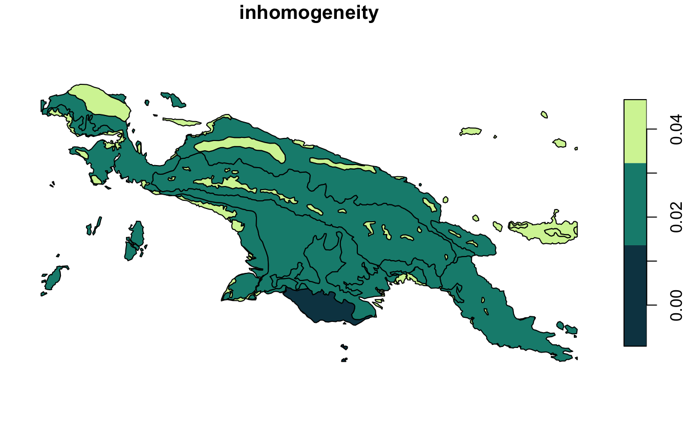
stars
To create a stars object with a new attribute
clust, we should set output = "stars".
However, it is not yet possible to calculate the quality of the
clustering for the stars objects.
landcover_grid_stars2 = lsp_add_clusters(landcover_cove2, clusters2,
                                         window = ecoregions["id"], output = "stars")
plot(landcover_grid_stars2["clust"], col = safe_pal4)
#> downsample set to 12