Spatial patterns’ search
Jakub Nowosad
2025-07-26
Source:vignettes/articles/v3_search.Rmd
v3_search.RmdThe pattern-based spatial analysis makes it possible to search for areas with similar spatial patterns. This vignette shows how to do spatial patterns’ search on example datasets. Let’s start by attaching necessary packages:
library(motif)
library(stars)
#> Loading required package: abind
#> Loading required package: sf
#> Linking to GEOS 3.13.0, GDAL 3.8.5, PROJ 9.5.1; sf_use_s2() is TRUE
library(sf)
library(tmap)
Spatial patterns’ search requires two spatial objects. The first one
is the area of interest, and the second one is a larger area that we
want to search in. For this vignette, we read the
"raster/landcover2015.tif" file, and crop our area of
interest using coordinates of its borders.
landcover = read_stars(system.file("raster/landcover2015.tif", package = "motif"))
ext = st_bbox(c(xmin = 238000, xmax = 268000,
ymin = -819814, ymax = -789814),
crs = st_crs(landcover))
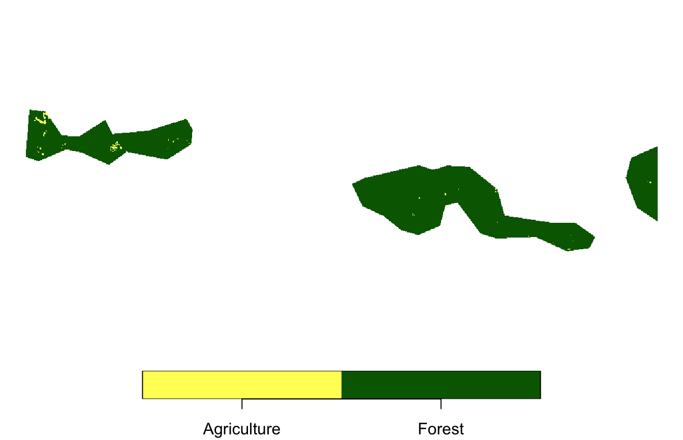
landcover_ext = landcover[ext]The landcover_ext represents area mostly covered by
forest with some agriculture.
We want to compare it to the land cover dataset of New Guinea -
landcover.
#> downsample set to 12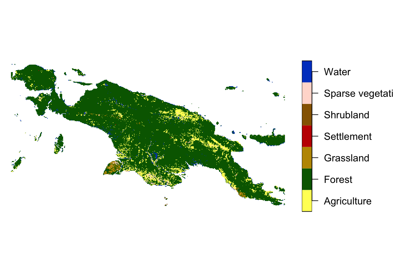
Regular local landscapes
Spatial patterns’ search is done by the lsp_search()
function. It expects an area of interest as the first object and the
larger area as the second one. We should provide the type of signature
(type) and the suitable distance function
(dist_fun) that we want to use to compare two datasets.
Additional arguments include the size of the search window from the
larger area (window) and how much of NA values we can
accept in the local landscapes (threshold).
search_1 = lsp_search(landcover_ext, landcover,
                      type = "cove", dist_fun = "jensen-shannon",
                      window = 100, threshold = 1)
search_1
#> stars object with 2 dimensions and 3 attributes
#> attribute(s):
#>                  Min.      1st Qu. Median         Mean 3rd Qu. Max.
#> id       1.0000000000 722.25000000 1443.5 1443.5000000 2164.75 2886
#> na_prop  0.0000000000   0.00220000    1.0    0.6757365    1.00    1
#> dist     0.0001794214   0.05387658    0.5    0.3352646    0.50    1
#> dimension(s):
#>   from to   offset  delta  refsys x/y
#> x    1 74 -1091676  30000 unnamed [x]
#> y    1 39   -38556 -30000 unnamed [y]
The result of the lsp_search() function is a
stars object with three attributes:
-
id- unique value for each local landscape -
na_prop- proportion (0-1) of NA values in each local landscapes -
dist- the distance between our area of interest and each local landscape
We can visualize the results, using, for example, the tmap package:
my_breaks = c(0, 0.001, 0.01, 0.1, 1.01)
tm_shape(search_1) +
  tm_raster("dist", breaks = my_breaks, palette = "-viridis") +
  tm_layout(legend.outside = TRUE)
#>
#> ── tmap v3 code detected ───────────────────────────────────────────────────────
#> [v3->v4] `tm_tm_raster()`: migrate the argument(s) related to the scale of the
#> visual variable `col` namely 'breaks', 'palette' (rename to 'values') to
#> col.scale = tm_scale(<HERE>).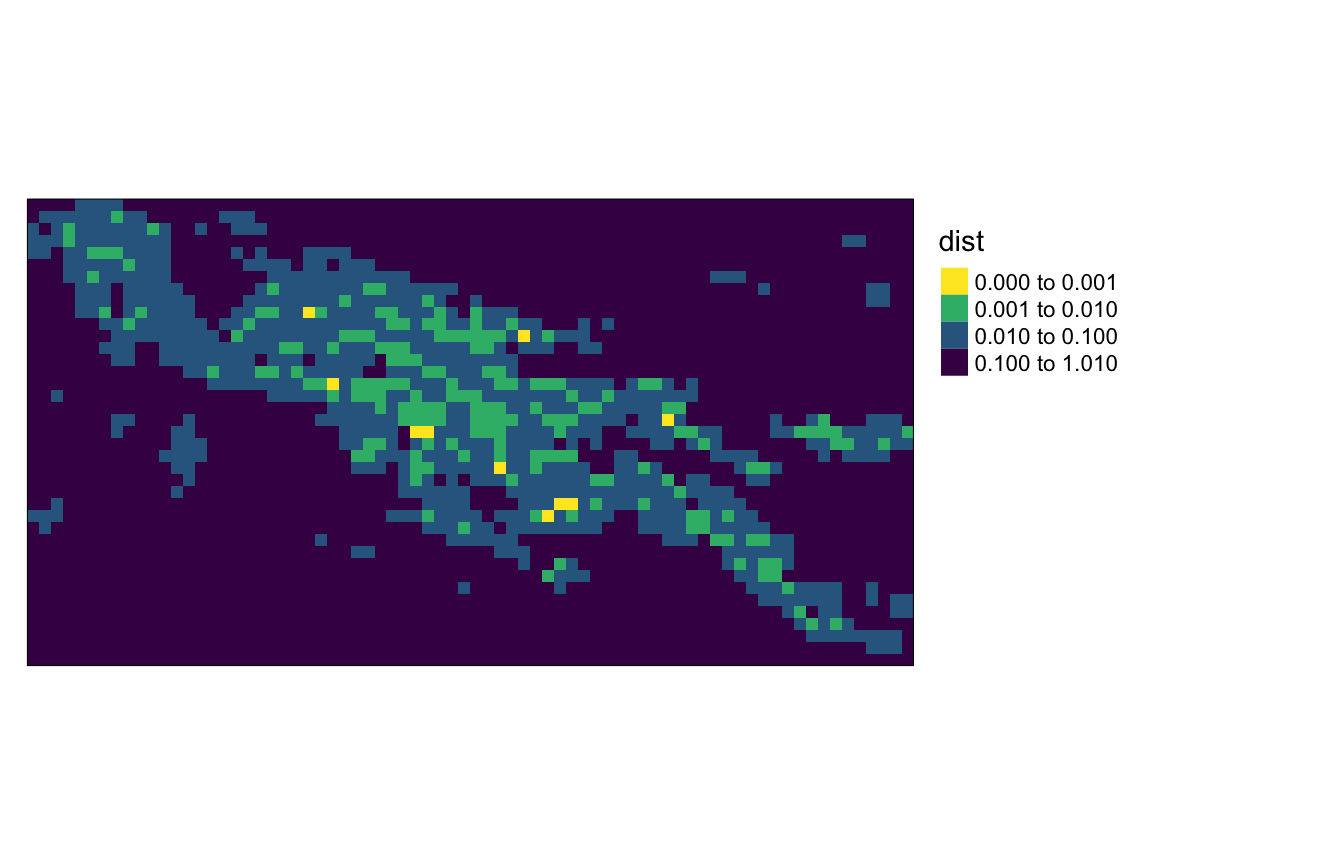
It is now possible to see that there are several areas with a
distance below 0.001 represented by a yellow color - they are the most
similar to landcover_ext.
We can find their ids using the code below.
unique(search_1$id[which(search_1$dist < 0.001)])
#>  [1]  690  856 1136 1386 1439 1440 1668 1895 1896 1968
To extract selected local landscape, the lsp_extract()
function can be used.
search_1_690 = lsp_extract(landcover,
window = 100,
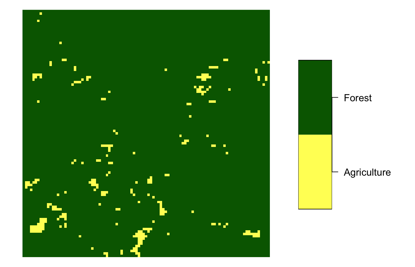
id = 690)Its output is a stars object, that we can vizualize and
see that it is fairly similar to the area of interest.
search_1_690 = droplevels(search_1_690)
plot(search_1_690, main = NULL)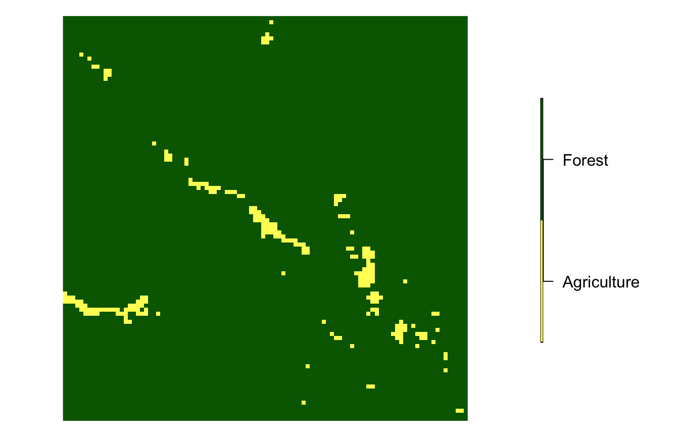
Irregular local landscapes
Search is also possible in irregular local landscapes, based on
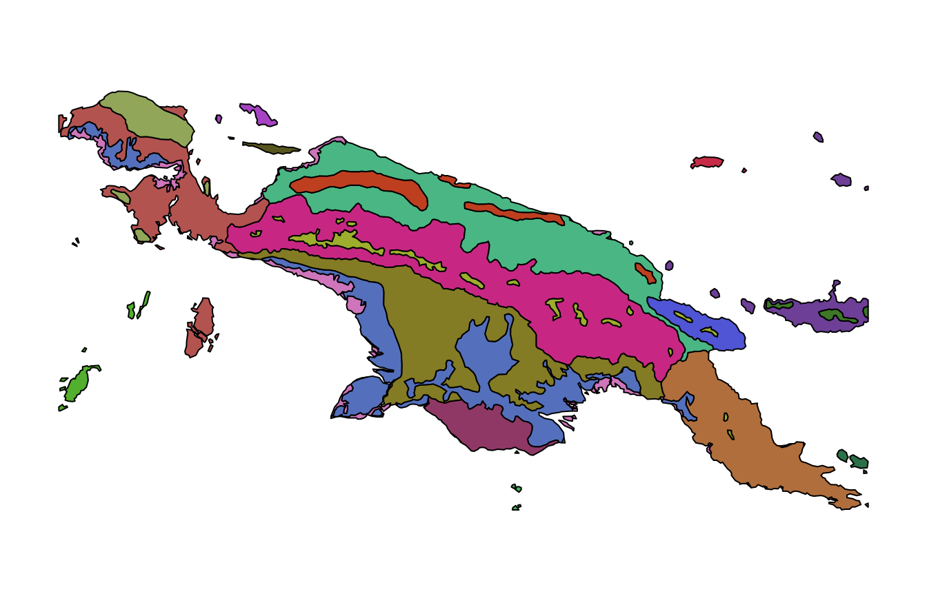
polygon data. ecoregions.gpkg contains terrestrial
ecoregions for New Guinea from https://ecoregions2017.appspot.com/.
ecoregions = read_sf(system.file("vector/ecoregions.gpkg", package = "motif"))This dataset has 22 rows, where each row relates to one ecoregion.
Each ecoregion is also related to a unique value in the id
column.
The lsp_search() function works very similarly to the
previous case - we just need to provide our ecoregions in the
window argument.
search_2 = lsp_search(landcover_ext, landcover,
                      type = "cove", dist_fun = "jensen-shannon",
                      window = ecoregions["id"], threshold = 1)
search_2
#> stars object with 2 dimensions and 3 attributes
#> attribute(s), summary of first 1e+05 cells:
#>                  Min.      1st Qu.       Median         Mean      3rd Qu.
#> id       21.000000000 21.000000000 21.000000000 21.000000000 21.000000000
#> na_prop   0.007177053  0.007177053  0.007177053  0.007177053  0.007177053
#> dist      0.016081750  0.016081750  0.016081750  0.016081750  0.016081750
#>                  Max.  NA's
#> id       21.000000000 98383
#> na_prop   0.007177053 98383
#> dist      0.016081750 98383
#> dimension(s):
#>   from   to   offset delta  refsys point x/y
#> x    1 7360 -1091676   300 unnamed FALSE [x]
#> y    1 3812   -38556  -300 unnamed FALSE [y]
Let’s vizualize the output:
my_breaks = c(0, 0.001, 0.01, 0.1, 1.01)
tm_shape(search_2) +
  tm_raster("dist", breaks = my_breaks, palette = "-viridis") +
  tm_shape(ecoregions) +
  tm_borders(col = "black") +
  tm_layout(legend.outside = TRUE)
#>
#> ── tmap v3 code detected ───────────────────────────────────────────────────────
#> [v3->v4] `tm_tm_raster()`: migrate the argument(s) related to the scale of the
#> visual variable `col` namely 'breaks', 'palette' (rename to 'values') to
#> col.scale = tm_scale(<HERE>).
#> stars object downsampled to 3680 by 1906 cells.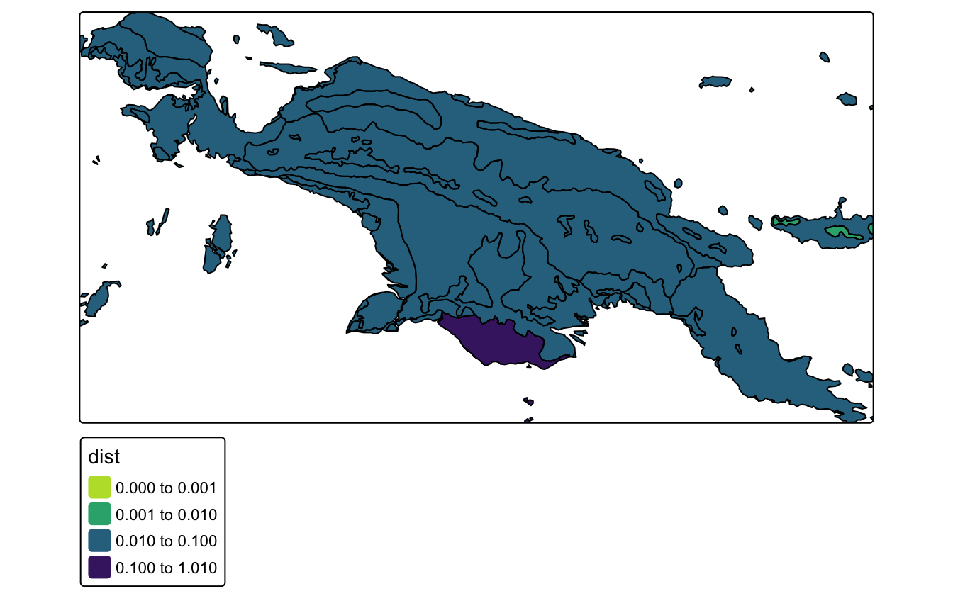
This search shows that most of the polygons are fairly different from our area of interest. Only one of them, located in the east, has a relatively small distance of about 0.007.
min_search2 = min(search_2$dist, na.rm = TRUE)
min_search2
#> [1] 0.006810959
We can obtain its id (10) using the code below.
Now, we can use lsp_extract() to extract land cover for
this ecoregion.
search_2_10 = lsp_extract(landcover,
                          window = ecoregions["id"],
                          id = 10)
This local landscape is also mostly covered by forest with just some smaller areas of agriculture.
search_2_10 = droplevels(search_2_10)
plot(search_2_10, main = NULL)