Search for similar spatial pattern — lsp

Searches for areas with similar spatial patterns in categorical data. It accepts a categorical raster dataset with one or more attributes, and compares it to the second (usually larger) dataset with the same attributes. The first dataset is either compared to a whole area, areas divided into regular windows, or areas divided into irregular windows from the second dataset. This function allows for several types of comparisons using different representations of spatial patterns, including "coma" (co-occurrence matrix), "cove" (co-occurrence vector), "cocoma" (co-located co-occurrence matrix), "cocove" (co-located co-occurrence vector), "wecoma" (weighted co-occurrence matrix), "wecove" (weighted co-occurrence vector), "incoma" (integrated co-occurrence matrix), "incove" (integrated co-occurrence vector). These representations are created for both datasets, and next a distance between them is calculated using a selected measure from the philentropy::distance function. Additional parameters, such as neighbourhood or normalization types, are also available.

lsp_search(
  x,
  y,
  type,
  dist_fun,
  window = NULL,
  output = "stars",
  neighbourhood = 4,
  threshold = 0.5,
  ordered = FALSE,
  repeated = FALSE,
  normalization = "pdf",
  wecoma_fun = "mean",
  wecoma_na_action = "replace",
  classes = NULL,
  ...
)

Arguments

x: Object of class stars, stars_proxy, or terra's SpatRaster. It should have one attribute (for "coma", "cove"), two attributes ("cocoma", "cocove", "wecoma", "wecove"), two or more attributes ("incoma", "incove"), or any number of attributes suitable for user-defined functions.
y: Object of class stars, stars_proxy, or terra's SpatRaster. It should have one attribute (for "coma", "cove"), two attributes ("cocoma", "cocove", "wecoma", "wecove"), two or more attributes ("incoma", "incove"), or any number of attributes suitable for user-defined functions.
type: Type of the calculated signature. It can be "coma" (co-occurrence matrix), "cove" (co-occurrence vector), "cocoma" (co-located co-occurrence matrix), "cocove" (co-located co-occurrence vector), "wecoma" (weighted co-occurrence matrix), "wecove" (weighted co-occurrence vector), "incoma" (integrated co-occurrence matrix), "incove" (integrated co-occurrence vector), "composition" or any function that can summarize stars objects.
dist_fun: Distance measure used. This function uses the philentropy::distance function in the background. Run philentropy::getDistMethods() to find possible distance measures.
window: Specifies areas for analysis. It can be either: NULL, a numeric value, or an sf object. If window=NULL calculations are performed for a whole area. If the window argument is numeric, it is a length of the side of a square-shaped block of cells. Expressed in the numbers of cells, it defines the extent of a local pattern. If an sf object is provided, each feature (row) defines the extent of a local pattern. The sf object should have one attribute (otherwise, the first attribute is used as an id).
output: The class of the output. Either "stars", "sf", or "terra"
neighbourhood: The number of directions in which cell adjacencies are considered as neighbours: 4 (rook's case) or 8 (queen's case). The default is 4.
threshold: The share of NA cells to allow metrics calculation.
ordered: For "cove", "cocove", "wecove" and "incove" only. The type of pairs considered. Either "ordered" (TRUE) or "unordered" (FALSE). The default is FALSE.
repeated: For "incove" only. Should the repeated co-located co-occurrence matrices be used? Either "ordered" (TRUE) or "unordered" (FALSE). The default is FALSE.
normalization: For "cove", "cocove", "wecove", "incove", "composition", or user-provided functions only. Should the output vector be normalized? Either "none" or "pdf". The "pdf" option normalizes a vector to sum to one. The default is "pdf".
wecoma_fun: For "wecoma" and "wecove" only. Function to calculate values from adjacent cells to contribute to exposure matrix, "mean" - calculate average values of local population densities from adjacent cells, "geometric_mean" - calculate geometric mean values of local population densities from adjacent cells, or "focal" assign a value from the focal cell
wecoma_na_action: For "wecoma" and "wecove" only. Decides on how to behave in the presence of missing values in w. Possible options are "replace", "omit", "keep". The default, "replace", replaces missing values with 0, "omit" does not use cells with missing values, and "keep" keeps missing values.
classes: Which classes (categories) should be analyzed? This parameter expects a list of the same length as the number of attributes in x, where each element of the list contains integer vector. The default is NULL, which means that the classes are calculated directly from the input data and all of them are used in the calculations.
...: Additional arguments for the philentropy::distance function.

Value

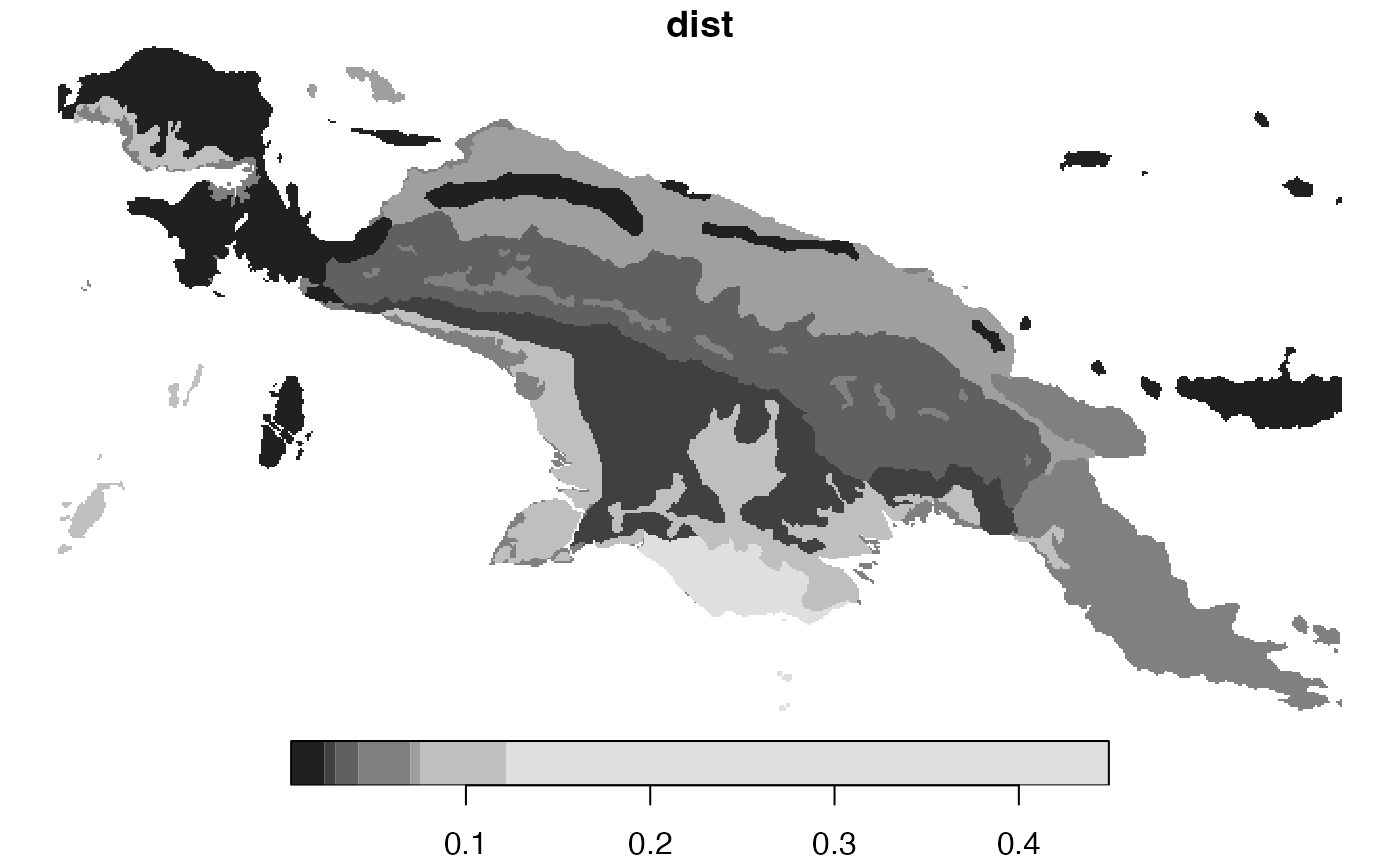
Object of class stars (or sf or terra's SpatRaster, depending on the output argument). It has three attributes: (1) id - an id of each window. For irregular windows, it is the values provided in the window argument, (2) na_prop - share (0-1) of NA cells for each window in the y object, (3) dist- calculated distance between the x object and each window in the y object

Examples

library(stars)

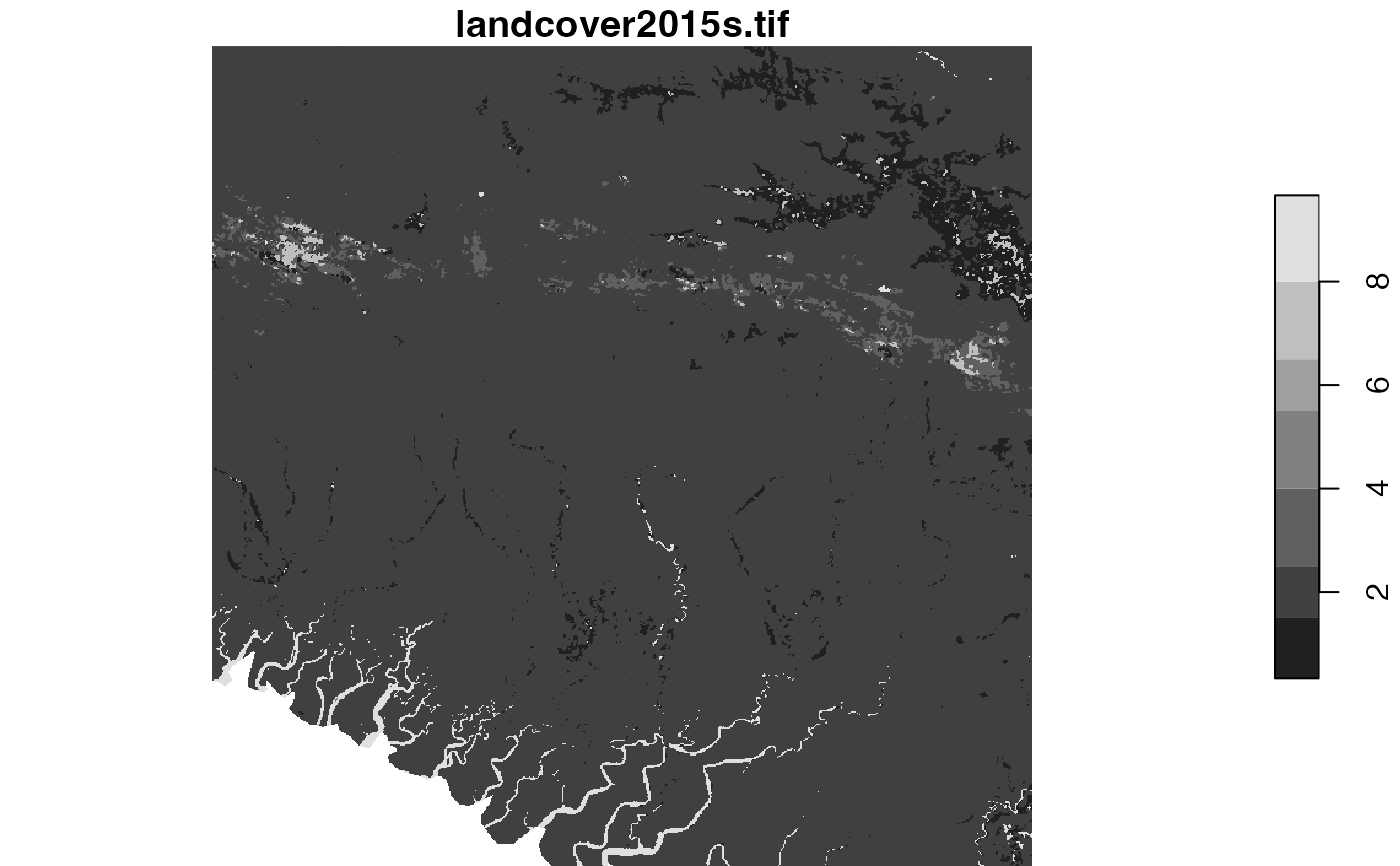
landcover = read_stars(system.file("raster/landcover2015s.tif", package = "motif"))
plot(landcover)


ext = st_bbox(c(xmin = -249797.344531127, xmax = -211162.693944285,
                ymin = -597280.143035389, ymax = -558645.492448547),
                crs = st_crs(landcover))

landcover_ext = landcover[ext]
plot(landcover_ext)


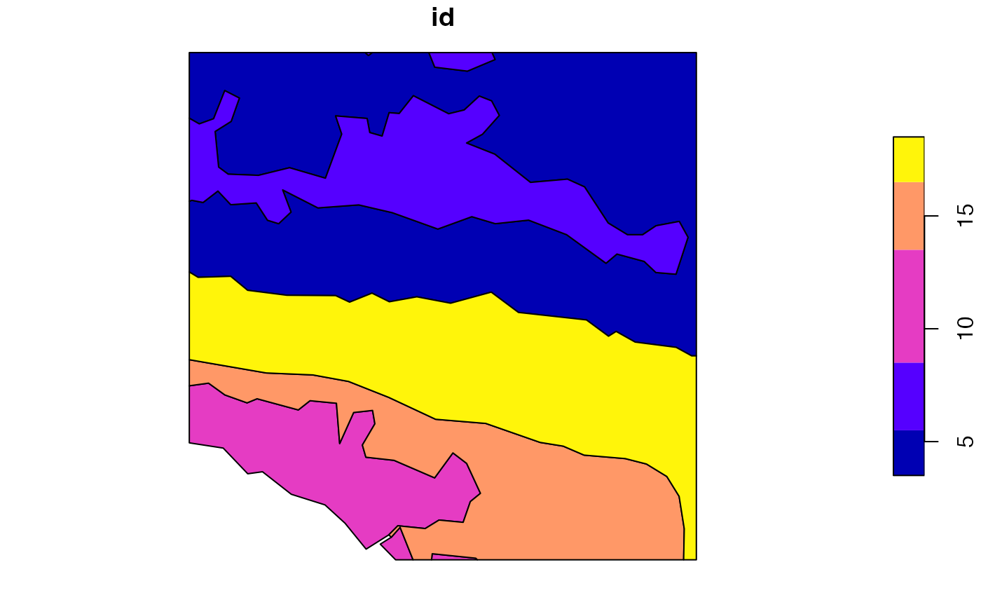
ecoregions = read_sf(system.file("vector/ecoregionss.gpkg", package = "motif"))
plot(ecoregions["id"])


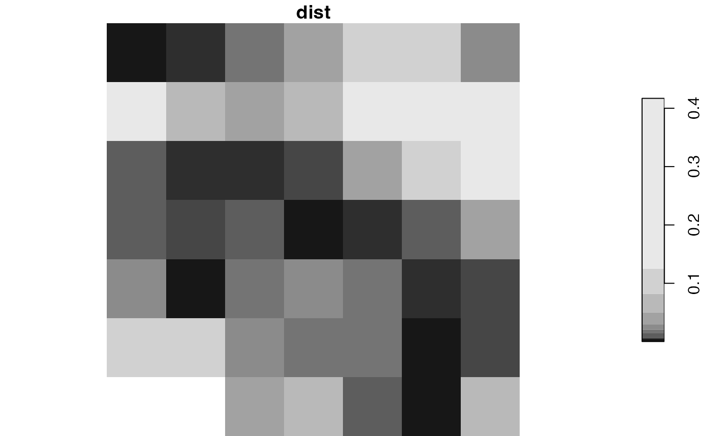
s1 = lsp_search(landcover_ext, landcover, type = "cove",
  dist_fun = "jensen-shannon", threshold = 0.9, window = 100)
plot(s1["dist"])


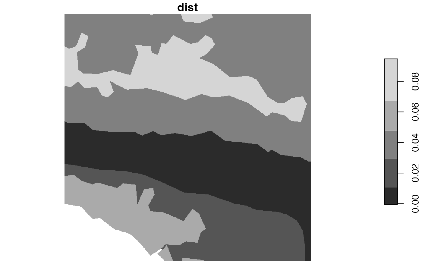
ecoregions = st_transform(ecoregions, st_crs(landcover))
s2 = lsp_search(landcover_ext, landcover, type = "cove",
  dist_fun = "jensen-shannon", threshold = 0.5, window = ecoregions["id"])
plot(s2["dist"])


# \donttest{
# larger data example
library(stars)

landcover = read_stars(system.file("raster/landcover2015.tif", package = "motif"))
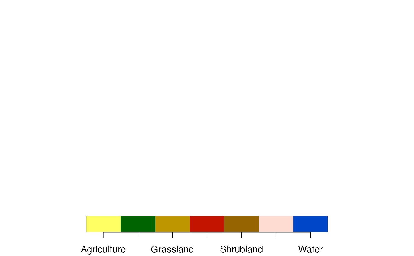
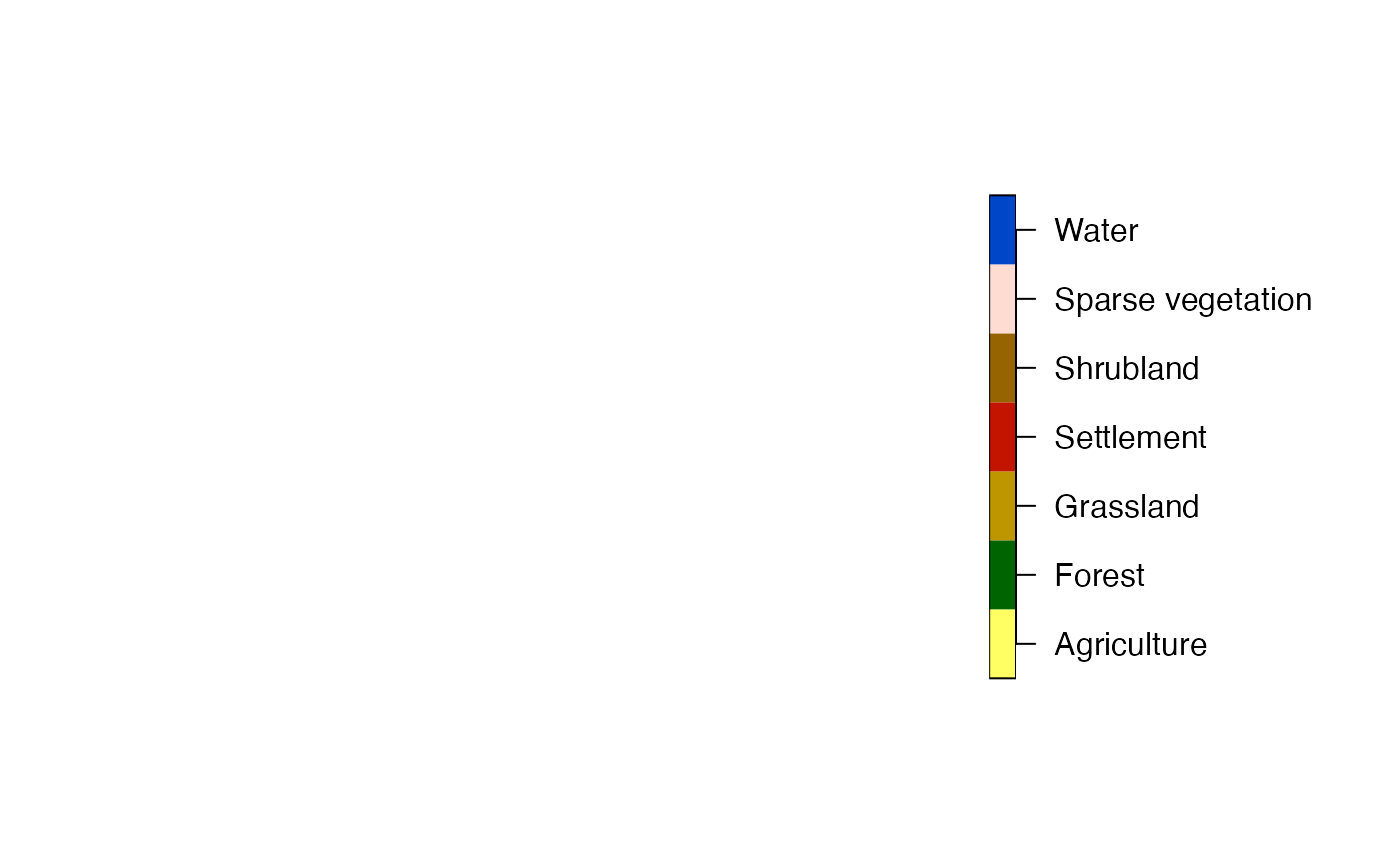
plot(landcover)
#> downsample set to 10
#> Error in image.stars(x, ..., axes = axes, breaks = breaks, col = col,     key.pos = key.pos, key.width = key.width, key.length = key.length,     main = NULL): rgb plotting not supported on this device

ext = st_bbox(c(xmin = -249797.344531127, xmax = -211162.693944285,
                ymin = -597280.143035389, ymax = -558645.492448547),
                crs = st_crs(landcover))

landcover_ext = landcover[ext]
plot(landcover_ext)

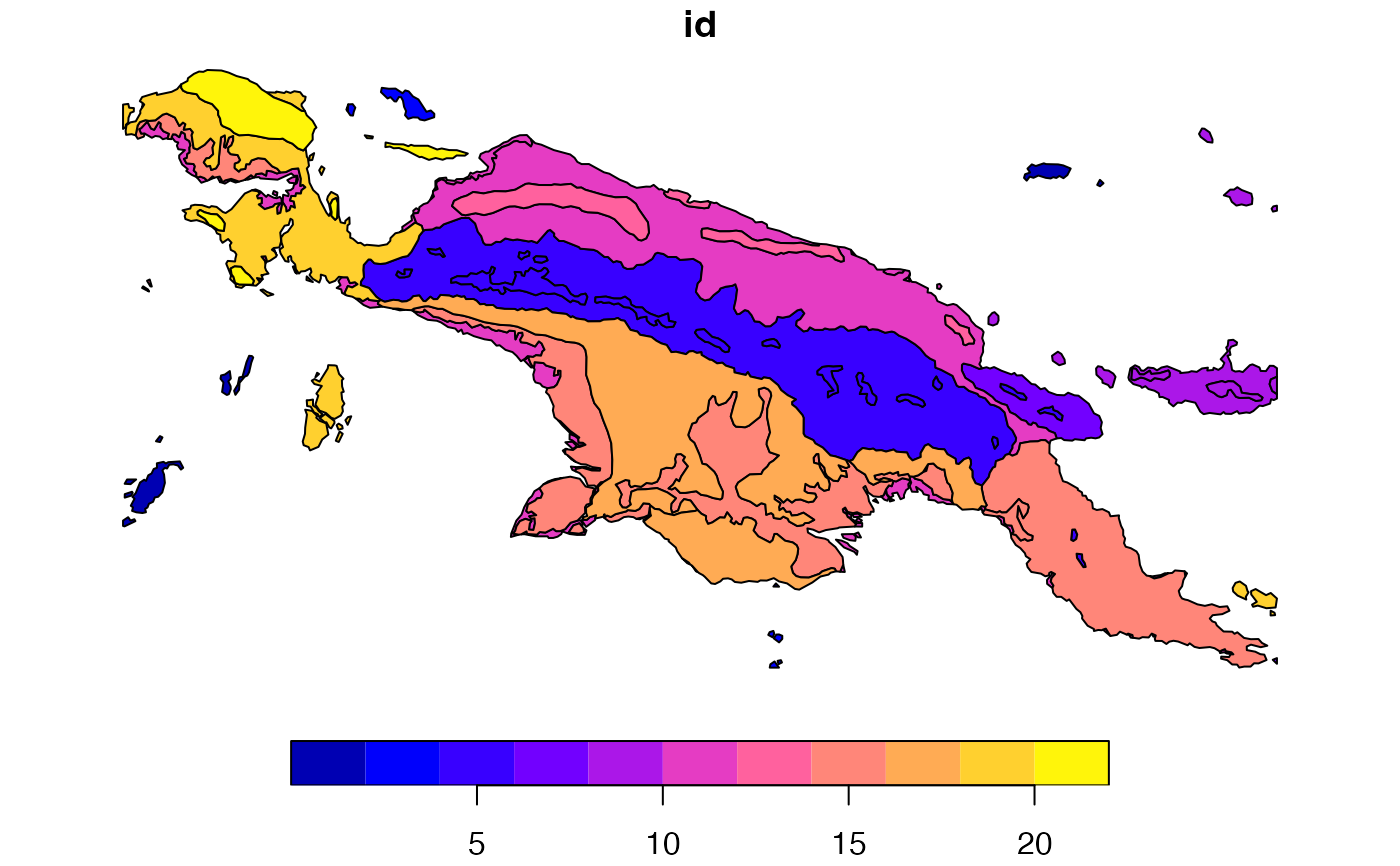
#> Error in image.stars(x, ..., axes = axes, breaks = breaks, col = col,     key.pos = key.pos, key.width = key.width, key.length = key.length,     main = NULL): rgb plotting not supported on this device

ecoregions = read_sf(system.file("vector/ecoregions.gpkg", package = "motif"))
plot(ecoregions["id"])



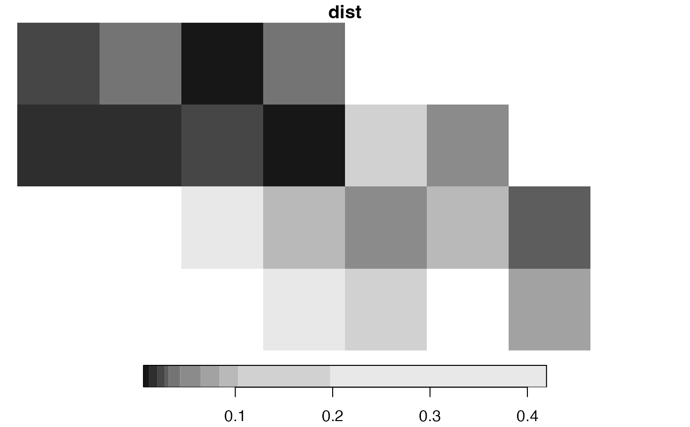
s1 = lsp_search(landcover_ext, landcover, type = "cove",
  dist_fun = "jensen-shannon", threshold = 0.9, window = 1000)
plot(s1["dist"])


ecoregions = st_transform(ecoregions, st_crs(landcover))
s2 = lsp_search(landcover_ext, landcover, type = "cove",
  dist_fun = "jensen-shannon", threshold = 0.5, window = ecoregions["id"])
plot(s2["dist"])
#> downsample set to 10

# }