Extracting the proportion of different classes in many regular local landscapes
Jakub Nowosad
2025-07-26
Source:vignettes/articles/v6_composition.Rmd
v6_composition.RmdThe pattern-based analysis, as explained in Nowosad (2021), is concerned with describing spatial patterns for many local landscapes - blocks of cells containing a local pattern of a cell-based variable(s). One of its core ideas is to transform information stored in each local landscape’s cells into a spatial signature — a statistical description of a pattern.
The proportion of different classes, also known as composition, can be considered as a basic spatial signature of categorical rasters. It is well-known that composition is a fundamental element of a landscape pattern (Riitters 2019), and for example, the proportion of different land cover classes has a significant impact on environmental processes.
The role of this vignette is to show how to calculate the proportion of different classes in many regular local landscapes using the motif package. Let’s start by attaching necessary packages:
For this vignette, we use the "raster/landcover2015.tif"
file, which contains land cover data for New Guinea, with seven possible
categories: (1) agriculture, (2) forest, (3) grassland, (5) settlement,
(6) shrubland, (7) sparse vegetation, and (9) water.
landcover = read_stars(system.file("raster/landcover2015.tif", package = "motif"))
landcover = droplevels(landcover)
plot(landcover, key.pos = 4, key.width = lcm(5), main = NULL)
#> downsample set to 12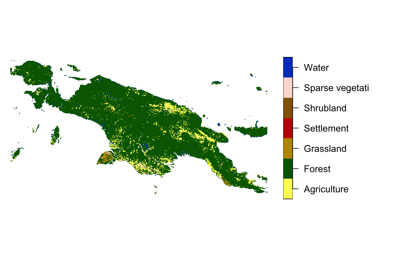
New grid
One possible approach is just to set up size of a local landscape in
the lsp_signature() function. For example,
window = 100 divides the input raster into a number of
non-overlapping 100 by 100 cells local landscapes. To extract the
proportion of different classes in the landcover raster, we
need to set type to "composition"1.
landcover_comp = lsp_signature(landcover,
                               type = "composition",
                               threshold = 1,
                               window = 100)
Information about the composition of each local landscape is stored
in a list-column named signature.
landcover_comp
#> # A tibble: 2,886 × 3
#>       id na_prop signature
#>  * <int>   <dbl> <list>
#>  1     1  0.982  <dbl [1 × 7]>
#>  2     2  0.978  <dbl [1 × 7]>
#>  3     3  1      <dbl [1 × 7]>
#>  4     4  0.934  <dbl [1 × 7]>
#>  5     5  0.357  <dbl [1 × 7]>
#>  6     6  0.0398 <dbl [1 × 7]>
#>  7     7  0.114  <dbl [1 × 7]>
#>  8     8  0.465  <dbl [1 × 7]>
#>  9     9  0.884  <dbl [1 × 7]>
#> 10    10  1      <dbl [1 × 7]>
#> # ℹ 2,876 more rows
Objects of this structure can be next used in many spatial
pattern-based analysis, such as search,
comparision,
or clustering.
However, it could be useful for some operations to have each proportion
as a separate column. This can be done with the
lsp_restructure() function.
landcover_comp = lsp_restructure(landcover_comp)Now, each land cover category has a separate column, but the columns’
names are meaningless. To add column names representing actual land
cover categories, we can extract correct names from the
landcover_comp object attributes.
true_colnames = attr(landcover_comp, "metadata")$vals[[1]]
names(landcover_comp)[3:ncol(landcover_comp)] = true_colnames
landcover_comp
#> # A tibble: 2,886 × 9
#>       id na_prop        `1`     `2`   `3`        `4`   `5`   `6`      `7`
#>  * <int>   <dbl>      <dbl>   <dbl> <dbl>      <dbl> <dbl> <dbl>    <dbl>
#>  1     1  0.982    0          0.5       0   0            0     0   0.5
#>  2     2  0.978    0          0.568     0   0            0     0   0.432
#>  3     3  1      NaN        NaN       NaN NaN          NaN   NaN NaN
#>  4     4  0.934    0          0.691     0   0            0     0   0.309
#>  5     5  0.357    0.000311   0.958     0   0.000778     0     0   0.0408
#>  6     6  0.0398   0.000833   0.977     0   0            0     0   0.0226
#>  7     7  0.114    0.000452   0.965     0   0            0     0   0.0341
#>  8     8  0.465    0          0.877     0   0            0     0   0.123
#>  9     9  0.884    0.0344     0.552     0   0.000861     0     0   0.412
#> 10    10  1      NaN        NaN       NaN NaN          NaN   NaN NaN
#> # ℹ 2,876 more rows
The above result is a special data frame of class lsp.
This allows us to easily add spatial information about the borders of
the local landscapes with lsp_add_sf().
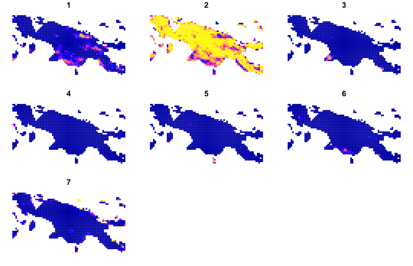
landcover_comp_sf = lsp_add_sf(landcover_comp) # this function adds our grid as an sf objectNow, the proportions of land cover categories can be visualized with
the plot() function 2. All categories:
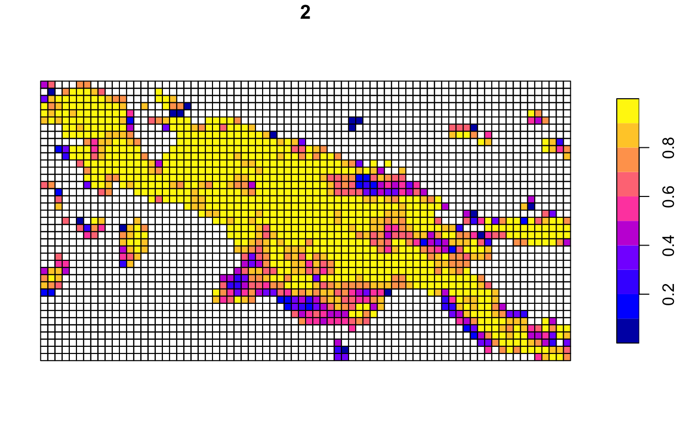
Just the second category - forest:
plot(landcover_comp_sf["2"])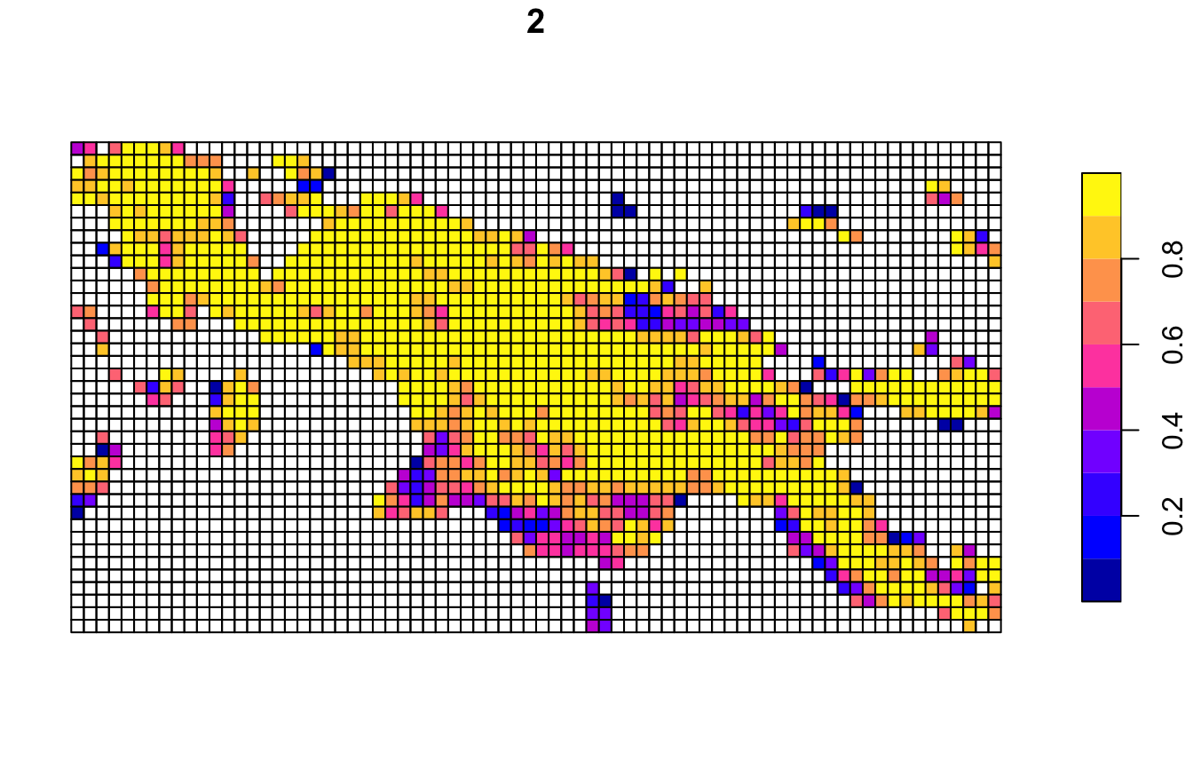
Existing areas
The second approach is to create or use existing local landscape
areas in the form of an sf polygons. Importantly, this
approach could be visibly slower - therefore, if your local landscapes
are represented by a regular grid, we recommend using the first
approach.
For example, here, we create a my_grid object - a set of
sf polygons, where each polygon has a size of 30 by 30 km
and a unique id column.
my_grid = st_make_grid(landcover, cellsize = 30000)
my_grid = st_sf(data.frame(id = seq(length(my_grid), 1, by = -1)), geom = my_grid)
plot(my_grid)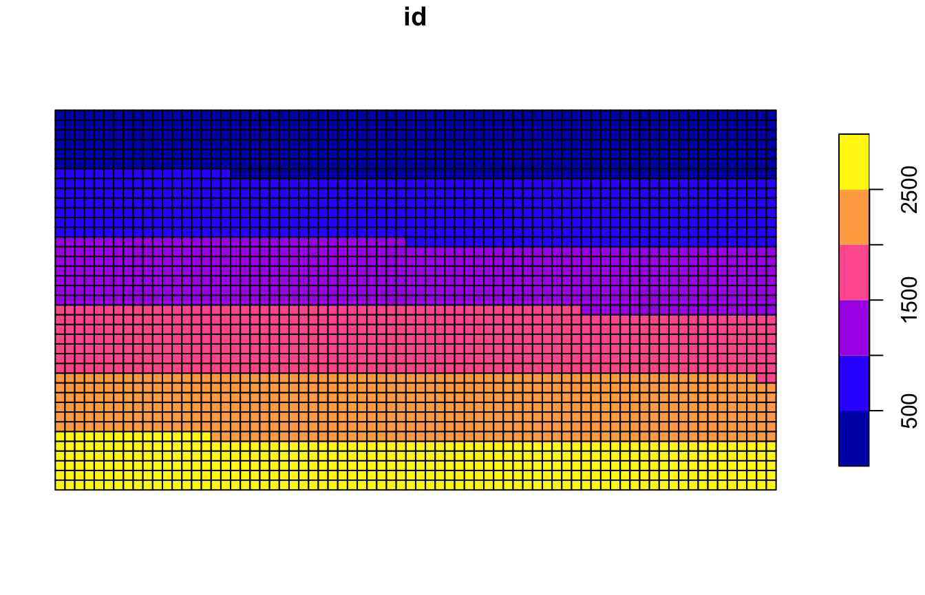
The next steps are the same as in the first approach - we use the
lsp_signature(), lsp_restructure(), and
lsp_add_sf() functions. There are only two slight
differences. Firstly, we use our my_grid object as the
value of the window argument.
landcover_comp2 = lsp_signature(landcover,
                               type = "composition",
                               threshold = 1,
                               window = my_grid)
landcover_comp2 = lsp_restructure(landcover_comp2)
names(landcover_comp2)[3:ncol(landcover_comp2)] = attr(landcover_comp2, "metadata")$vals[[1]]
landcover_comp2
#> # A tibble: 2,886 × 9
#>       id na_prop   `1`   `2`   `3`   `4`   `5`   `6`   `7`
#>  * <int>   <dbl> <dbl> <dbl> <dbl> <dbl> <dbl> <dbl> <dbl>
#>  1     1       1   NaN   NaN   NaN   NaN   NaN   NaN   NaN
#>  2     2       1   NaN   NaN   NaN   NaN   NaN   NaN   NaN
#>  3     3       1   NaN   NaN   NaN   NaN   NaN   NaN   NaN
#>  4     4       1   NaN   NaN   NaN   NaN   NaN   NaN   NaN
#>  5     5       1   NaN   NaN   NaN   NaN   NaN   NaN   NaN
#>  6     6       1   NaN   NaN   NaN   NaN   NaN   NaN   NaN
#>  7     7       1   NaN   NaN   NaN   NaN   NaN   NaN   NaN
#>  8     8       1   NaN   NaN   NaN   NaN   NaN   NaN   NaN
#>  9     9       1   NaN   NaN   NaN   NaN   NaN   NaN   NaN
#> 10    10       1   NaN   NaN   NaN   NaN   NaN   NaN   NaN
#> # ℹ 2,876 more rows
The second difference is when we want to convert our results to a
spatial object. In this case, we need to provide our
my_grid object as the value of the window
argument in lsp_add_sf().
Proportions of each land cover categories:
landcover_comp_sf2 = lsp_add_sf(landcover_comp2, window = my_grid)
plot(landcover_comp_sf2[-c(1, 2)], border = NA)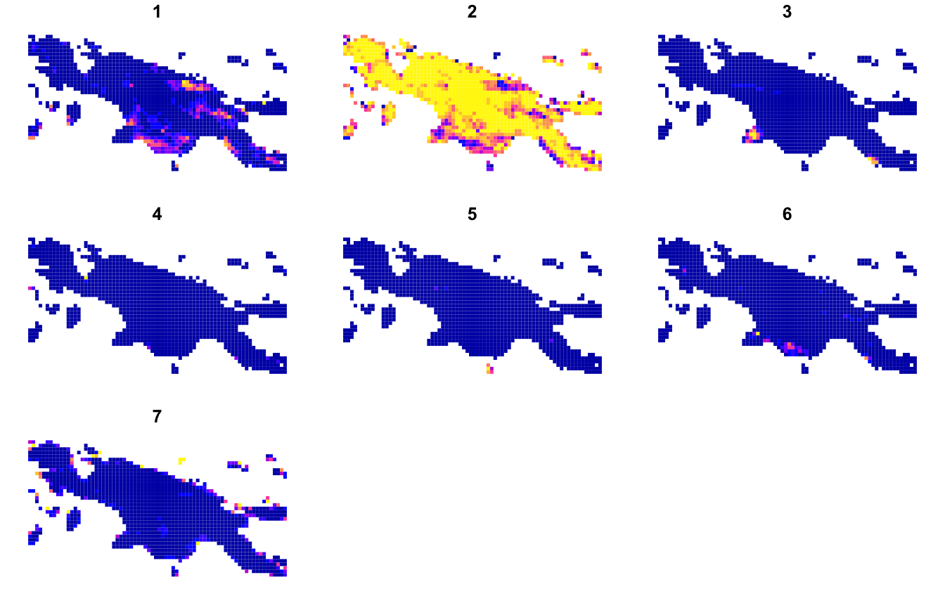
Just the second category - forest:
plot(landcover_comp_sf2["2"])