Choosing a distance measure for supercells

The distance measure defines what it means for the values of two raster cells to be similar. Therefore, the choice of a distance measure is crucial for the supercell segmentation results, and the decision of which measure to use should be based on the characteristics of the input data and the goals of the analysis. This vignette provides an overview of the available distance measures, their requirements, and guidance for selecting an appropriate measure for your analysis. It also includes a short example comparing three different measures on a sample raster dataset.

library(supercells)
library(terra)

Available measures

To check the available distance measures, use the sc_list_distances() function. It returns a data frame with information on the measure names, required input domains, what the measure compares, the effect of layer rescaling, and guidance for choosing the measure. Below is a summary of the available measures, grouped by input domain. The “Layer rescaling” column indicates whether differences in scale among layers affect the distance.

Input: Numeric Values

Name	What it compares	Layer rescaling	Guidance
euclidean	root-sum-square layer differences	can change distance	Scale layers to comparable units or ranges.
squared_euclidean	summed squared layer differences	can change distance	Scale layers to comparable units or ranges.
manhattan	summed absolute layer differences	can change distance	Scale layers to comparable units or ranges.
chebyshev	largest absolute layer difference	can change distance	Scale layers to comparable units or ranges.
canberra	relative layer differences	no effect	Layer scaling has no effect.
lorentzian	summed log-scaled layer differences	can change distance	Scale layers to comparable units or ranges.
cosine_distance	pattern across layers, ignoring overall scale	can change distance	Scale layers only to change their influence.

Input: Nonnegative Values

Name	What it compares	Layer rescaling	Guidance
soergel	difference relative to larger values	can change distance	Scale layers to set their influence.
wavehedges	summed relative layer differences	no effect	Layer scaling has no effect.
czekanowski	difference relative to total magnitude	can change distance	Scale layers to set their influence.
squared_chord	differences after square-root transformation	can change distance	Scale layers to set their influence.
squared_chi	squared differences relative to combined values	can change distance	Scale layers to set their influence.
clark	combined relative layer differences	no effect	Layer scaling has no effect.

Input: Probabilities Summing to 1

Name	What it compares	Layer rescaling	Guidance
jsd	difference between probability profiles	requires renormalization	Normalize every cell to sum to 1 and use mean centres.
non-intersection	probability assigned differently across layers	requires renormalization	Normalize every cell to sum to 1 and use mean centres.

Input: Probabilities in Equal-Width Bins Summing to 1

Name	What it compares	Layer rescaling	Guidance
wasserstein1	probability mass shifted across ordered bins	requires renormalization	Normalize every cell to sum to 1, use mean centres, and arrange layers in bin order.

Input: Ordered Numeric Sequence

Name	What it compares	Layer rescaling	Guidance
dtw	sequence difference after alignment	can change distance	Arrange layers in sequence order.

Input: Two Equal-Length Coordinate Sequences

Name	What it compares	Layer rescaling	Guidance
dtw2d	2D trajectory difference after alignment	can change distance	Arrange layers by dimension, with sequence order within each dimension.

Comparing three measures

We illustrate segmentations obtained with three distance measures: euclidean, canberra, and cosine_distance. Each measure is tuned separately because their distance values have different scales.

ortho <- rast(system.file("raster/ortho.tif", package = "supercells"))
ortho <- aggregate(ortho, fact = 2)

tune_euclidean <- sc_tune_compactness(ortho, step = 10, dist_fun = "euclidean")
sc_euclidean <- sc_slic(
  ortho,
  step = 10,
  compactness = tune_euclidean$compactness,
  dist_fun = "euclidean"
)

tune_canberra <- sc_tune_compactness(ortho, step = 10, dist_fun = "canberra")
sc_canberra <- sc_slic(
  ortho,
  step = 10,
  compactness = tune_canberra$compactness,
  dist_fun = "canberra"
)

tune_cosine <- sc_tune_compactness(ortho, step = 10, dist_fun = "cosine_distance")
sc_cosine <- sc_slic(
  ortho,
  step = 10,
  compactness = tune_cosine$compactness,
  dist_fun = "cosine_distance"
)

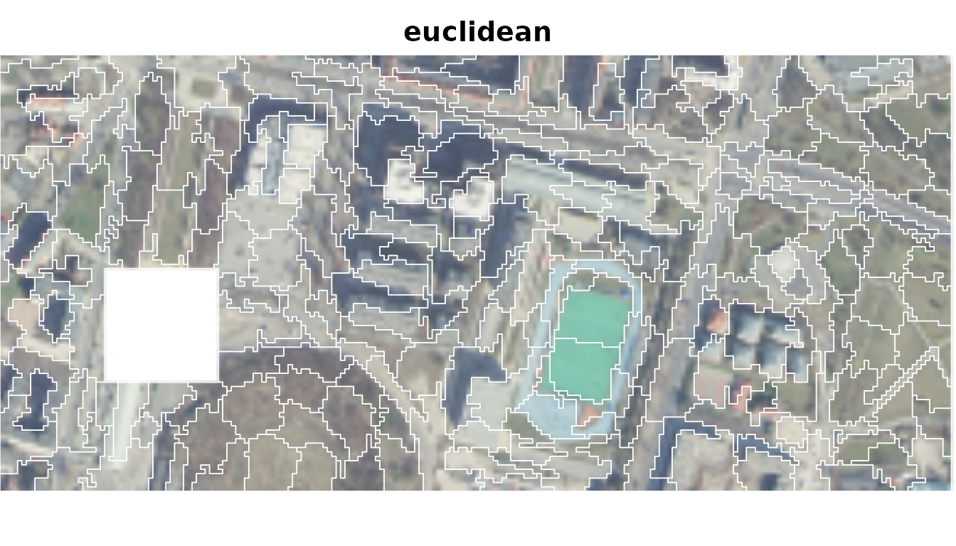
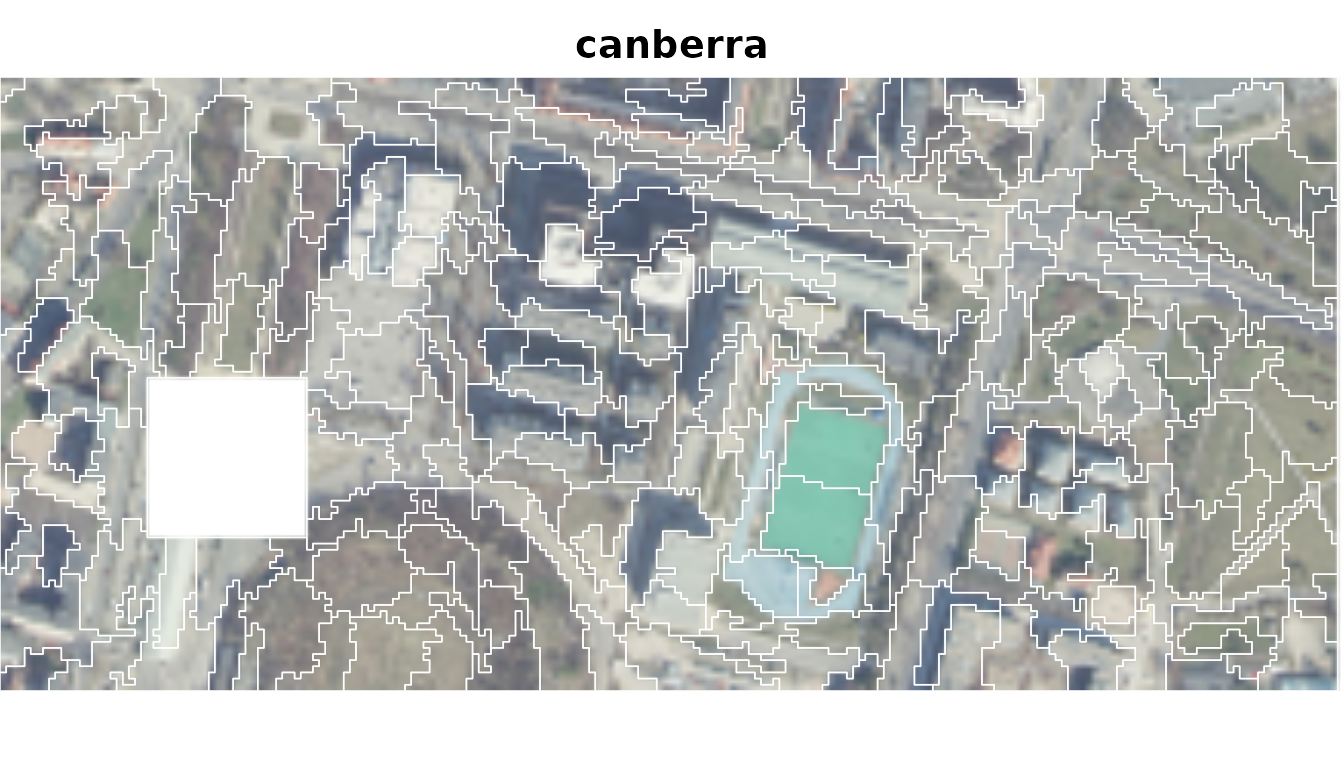
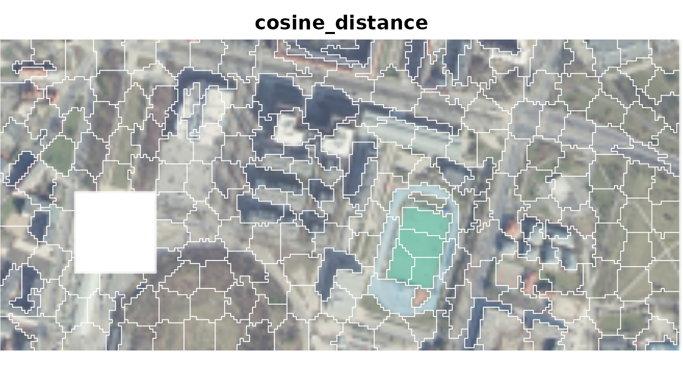
Each measure produces a different segmentation of the raster dataset:

Euclidean distance responds to absolute RGB differences.
Canberra distance compares channel differences relative to their values.
Cosine distance compares the RGB profile while ignoring its overall magnitude.

Custom measures

Other measures can be supplied as functions. A custom function must take two numeric vectors and return one finite, nonnegative value, with smaller values meaning greater similarity.

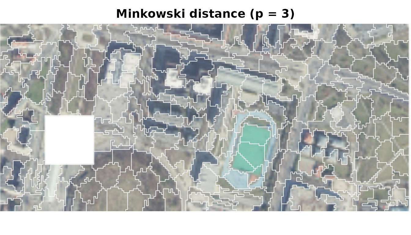
For example, Minkowski distance with $p = 3$ gives large layer differences more influence than Euclidean distance ( $p = 2$ ); Chebyshev distance is the limiting case as $p$ approaches infinity.

minkowski3 <- function(x, y) {
  sum(abs(x - y)^3)^(1 / 3)
}

tune_minkowski3 <- sc_tune_compactness(
  ortho,
  step = 10,
  dist_fun = minkowski3
)

sc_minkowski3 <- sc_slic(
  ortho,
  step = 10,
  compactness = tune_minkowski3$compactness,
  dist_fun = minkowski3
)

Jakub Nowosad

2026-11-07