Introduction to supercells

Jakub Nowosad

2026-02-09

The supercells package creates compact, homogeneous regions from raster data. It replaces thousands or millions of pixels with a smaller number of meaningful spatial units. This helps with interpretation, visualization, and downstream modeling. It also reduces noise while preserving important spatial structure.

The package is designed to work with rasters that have many layers or time steps. It supports multiple distance measures such as Jensen–Shannon divergence or dynamic time warping, as well as user-defined distance functions, so similarity can be adapted to the data. It can therefore handle diverse data types and high-dimensional inputs without changing the main workflow. The package core ideas are described in Nowosad and Stepinski (2022).

Core functions

The main function in the package is sc_slic(). It implements a SLIC-style algorithm that balances spatial compactness with value similarity (Achanta et al. 2012) and extends it to work with multi-layer rasters and custom distance functions. The output is a set of polygon supercells stored as an sf object. This object can include centers, average values, and IDs depending on the requested outcomes. In practice, sc_slic() is the entry point for most workflows.

The key tuning arguments in sc_slic() are step and compactness. step sets the spacing of initial centers and controls the expected number of supercells. It can be thought of as the expected spatial scale of the output. compactness controls the tradeoff between spatial regularity and value similarity. Lower values prioritize value similarity and may lead to irregular shapes, while higher values prioritize shape regularity – supercells may look more like squares – but may be less homogeneous in terms of values.

For compactness selection, you may use sc_tune_compactness() to estimate a good value from a short pilot run. Alternatively, compactness = use_adaptive() enables SLIC0-style adaptive compactness when you want the algorithm to adjust locally – this does not require setting a specific value, but also takes away direct control.

To assess quality of the resulting supercells, use sc_metrics_pixels() for pixel-level distances, sc_metrics_supercells() for per-supercell summaries, and sc_metrics_global() for a general overview. These metrics help compare different parameter settings or input preprocessing choices.

Workflow summary

Basic workflows follow the same pattern: choose scale (step or k), tune or set compactness, create supercells, and evaluate.

# read data
vol <- terra::rast(system.file("raster/volcano.tif", package = "supercells"))

# choose scale and tune compactness
tune <- supercells::sc_tune_compactness(vol, step = 8, metric = "local")

# create supercells
vol_sc <- supercells::sc_slic(vol, step = 8, compactness = tune$compactness)

# evaluate
metrics_global <- supercells::sc_metrics_global(vol, vol_sc)

Minimal example

The goal of this example is to derive supercells from a raster and visualize them. For that purpose, we will use the built-in volcano dataset, which is a small raster of elevation values.

library(supercells)
library(terra)

vol <- terra::rast(system.file("raster/volcano.tif", package = "supercells"))

This raster has 5307 cells – a small number for demonstration, but the same workflow applies to much larger rasters as well. Moreover, it has only one layer – but the same functions can handle multi-layer rasters with any number of layers.

Below, we create supercells in three different formats: polygons, points, and raster IDs. The polygon supercells are the most common output. Here, we specified step = 8 which would result in supercells of approximately 8x8 cells in size if they were perfectly regular, but the actual shapes and sizes will depend on the data and the compactness setting. The compactness is set to 1 – the behavior of this parameter depends on many factors, including the range of values in the raster, their properties, and the selected distance measure.

# Polygon supercells (sf)
vol_sc <- sc_slic(
  vol,
  step = 8,
  compactness = 1
)

terra::plot(vol)
plot(sf::st_geometry(vol_sc), add = TRUE, lwd = 0.6, border = "red")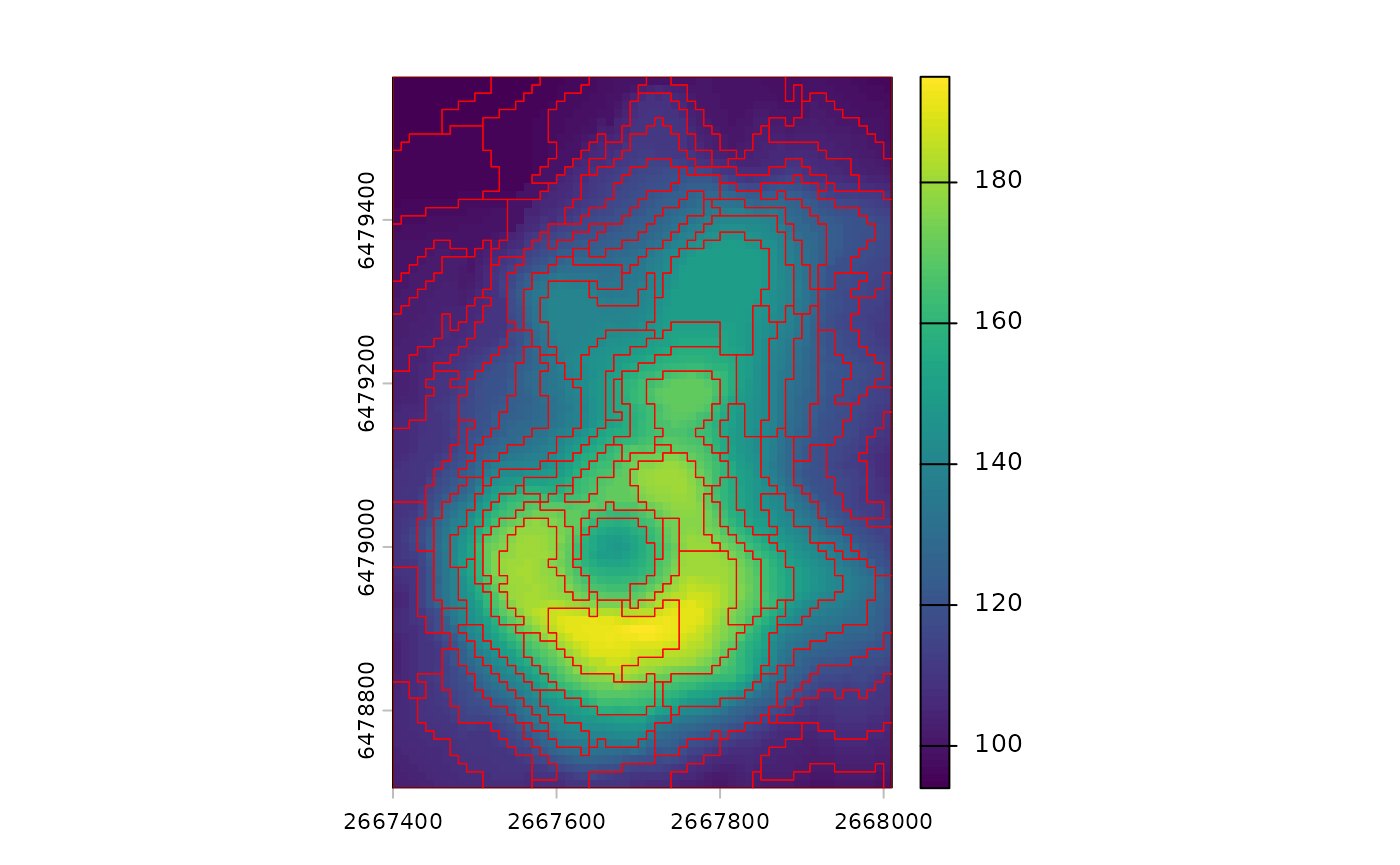

The resulting sf object contains one row per supercell. Each row stores summary values of each layer in the original raster, as well as the geometry of the supercell. By default, IDs, center coordinates, and summary values are returned (outcomes = c("supercells", "coordinates", "values")). Use outcomes = "values" when you want value summaries only.

Two related functions provide alternative output formats. Use sc_slic_points() to return only supercell centers as points. Use sc_slic_raster() to return a raster of supercell IDs for large datasets or raster-based pipelines. These functions share the same core arguments and can be swapped with minimal changes.

Now, let’s try to tune the compactness parameter using a pilot run.

tune <- sc_tune_compactness(
  vol,
  step = 8,
  metric = "local"
)
tune
#>   step metric  dist_fun compactness
#> 1    8  local euclidean    9.084872

Next, we may try to create supercells with the suggested compactness value.

vol_sc_tuned <- sc_slic(
  vol,
  step = 8,
  compactness = tune$compactness
)

terra::plot(vol)
plot(sf::st_geometry(vol_sc_tuned), add = TRUE, lwd = 0.6, border = "red")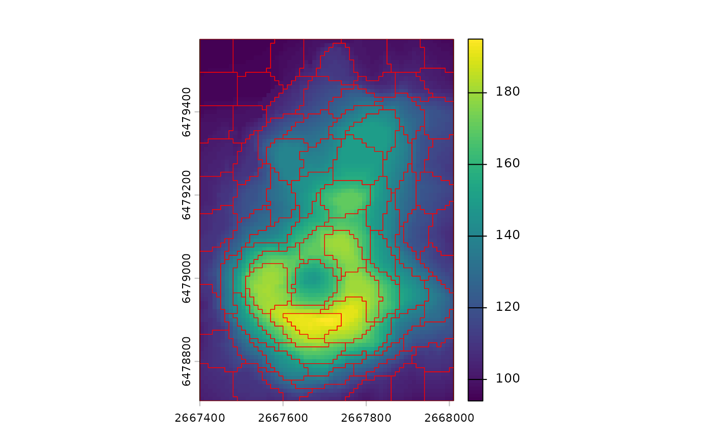

Such a derived compactness value may serve as a good starting point for further experimentation.

Afterwards, we can evaluate the quality of the resulting supercells using metrics on different levels.

pixel_metrics <- sc_metrics_pixels(vol, vol_sc_tuned)
supercell_metrics <- sc_metrics_supercells(vol, vol_sc_tuned)
global_metrics <- sc_metrics_global(vol, vol_sc_tuned)

The pixel-level metrics show how well the supercells represent the original raster values at the pixel level. By default they include spatial, value, combined, and balance. When scale = TRUE (the default), the spatial and value layers are returned as spatial_scaled and value_scaled.

plot(pixel_metrics, nr = 1)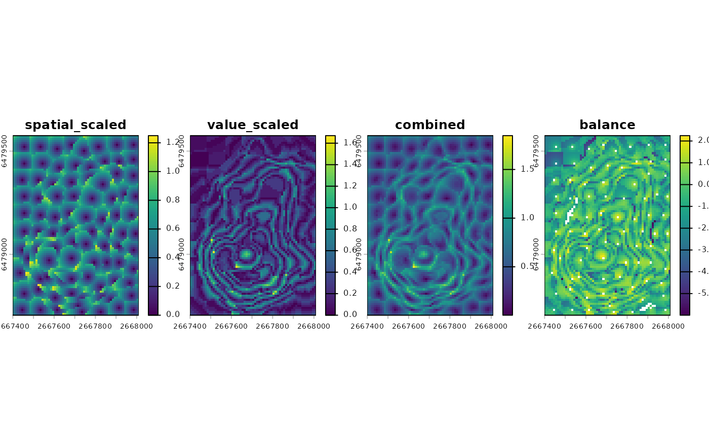

These maps help diagnose where spatial or value coherence is weak. For example, large patches of high values can indicate areas where the chosen parameters may be too coarse for local variation.

The supercell-level metrics summarize each polygon as a single value. These are helpful when you want to compare supercells or join metrics to attributes.

plot(supercell_metrics)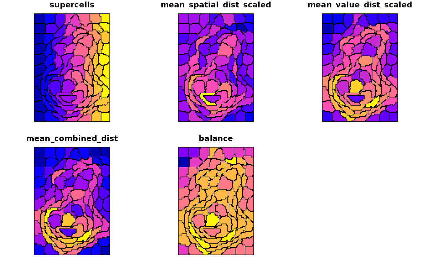

The global metrics provide a single-row summary of overall quality. They are useful for comparing parameter settings across multiple runs, such as a small grid of step and compactness values.

global_metrics
#>   step compactness adaptive_method n_supercells mean_spatial_dist_scaled
#> 1    8    9.084872            <NA>           88                0.4546412
#>   mean_value_dist_scaled mean_combined_dist    balance
#> 1              0.3061439          0.5915118 -0.4939904

Where to go next

To learn more about the package and its capabilities, check out the following articles:

• Choosing parameters: a practical guide to step, k, and compactness.
• Evaluation and diagnostics: how to read and compare pixel, supercell, and global metrics.
• Benchmarks: performance notes.
• Changes since v1: a concise summary of what’s new in v2.

References

Achanta, Radhakrishna, Appu Shaji, Kevin Smith, Aurelien Lucchi, Pascal Fua, and Sabine Süsstrunk. 2012. “SLIC Superpixels Compared to State-of-the-Art Superpixel Methods.” IEEE Transactions on Pattern Analysis and Machine Intelligence 34 (11): 2274–82.

Nowosad, Jakub, and Tomasz F. Stepinski. 2022. “Extended SLIC Superpixels Algorithm for Applications to Non-Imagery Geospatial Rasters.” International Journal of Applied Earth Observation and Geoinformation 112 (August): 102935. https://doi.org/10.1016/j.jag.2022.102935.