Choosing parameters for supercells

This vignette focuses on how parameters affect the supercell output, with the main choices being step or k, the compactness value, and the distance and averaging functions. The goal is not to find one universal set of parameters, but to choose values that match your intent.

All examples use the volcano raster for simplicity, but the same ideas apply to larger and multi-layer rasters.

library(supercells)
library(terra)

vol <- terra::rast(system.file("raster/volcano.tif", package = "supercells"))

Supercells algorithm

The supercells algorithm is an iterative process that starts with initial centers and assigns pixels to the nearest center based on a combined distance that incorporates both value similarity and spatial proximity. After the initial assignment, the algorithm updates the centers by averaging the values of the assigned pixels and recalculating the combined distance for the next iteration. This process continues until the specified number of iterations is reached.

In this package, the combined distance follows the standard SLIC form:

$D = \sqrt{\left(\frac{d_s}{\text{step}}\right)^2 + \left(\frac{d_v}{c}\right)^2}$

where $d_s$ is the spatial distance in grid-cell units, $d_v$ is the value-space distance (from dist_fun), and $c$ is the compactness value. When step is provided as use_meters(...), it is converted to cells before segmentation; distances are still computed in grid-cell units. Larger compactness down-weights the value term, making shapes more regular, while smaller values emphasize value similarity.

Choosing step or k

You can control the number and size of supercells using either step or k. step defines the spacing of initial centers in pixel units (or map units when given as use_meters(...)). Smaller step values produce more and smaller supercells, while larger values produce fewer and larger supercells. For example, step = 8 creates centers approximately every 8 pixels, which leads to supercells that are roughly 8 by 8 pixels in size, depending on the compactness.

sc_step <- sc_slic(vol, step = 8, compactness = 5)

By default, step is in pixel units, but instead we can also specify it in map units with use_meters(). This allows us to think about the spatial scales of expected supercells in terms of the actual map units. For example, if your raster has a resolution of 10 meters, then step = use_meters(200) would create centers approximately every 200 meters, which corresponds to every 20 pixels.

sc_step_map <- sc_slic(vol, step = use_meters(200), compactness = 5)

k specifies the desired number of supercells and the algorithm chooses an approximate step size. This is convenient when you want a target number instead of a target spatial scale.

sc_k <- sc_slic(vol, k = 100, compactness = 5)

In practice, use step when spatial scale matters, and use k when you want a fixed count across datasets. Importantly, both approaches still require a sensible compactness value.

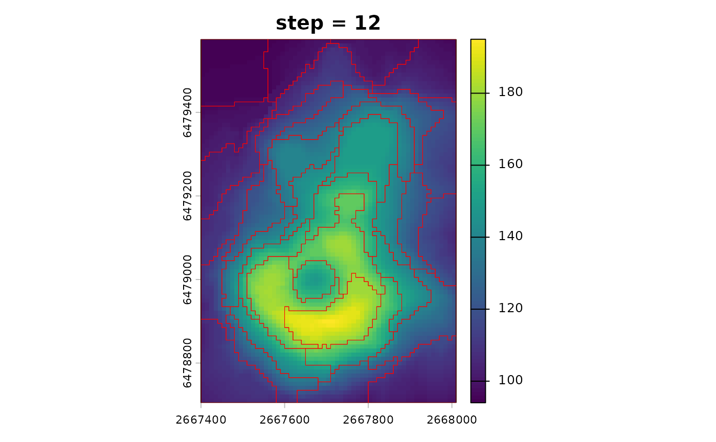
sc_step_small <- sc_slic(vol, step = 6, compactness = 5)
sc_step_large <- sc_slic(vol, step = 12, compactness = 5)
terra::plot(vol, main = "step = 6")
plot(sc_step_small[0], add = TRUE, border = "red", lwd = 0.5)
terra::plot(vol, main = "step = 12")
plot(sc_step_large[0], add = TRUE, border = "red", lwd = 0.5)

Choosing compactness

compactness controls the tradeoff between spatial regularity and value similarity: lower values favor value similarity and may create irregular shapes, while higher values favor more regular shapes but can mix dissimilar values.

In general, it is hard to predict the best compactness value without testing, and it depends on many factors including the range and distribution of values in your raster, the selected distance function, and the spatial structure of the data.

You can see this tradeoff by comparing two compactness values with the same step.

sc_compact_low <- sc_slic(vol, step = 8, compactness = 1)
sc_compact_high <- sc_slic(vol, step = 8, compactness = 10)
terra::plot(vol, main = "compactness = 1")
plot(sc_compact_low[0], add = TRUE, border = "red", lwd = 0.5)
terra::plot(vol, main = "compactness = 10")
plot(sc_compact_high[0], add = TRUE, border = "red", lwd = 0.5)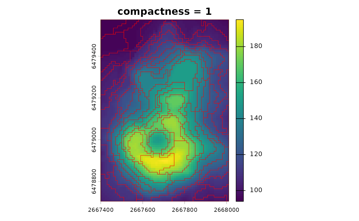

Tuning compactness

The sc_tune_compactness() function estimates a reasonable starting value from a short run of the algorithm.

It supports two summaries with metric = "global" and metric = "local". The global version looks at overall balance between value and spatial distances, while the local version uses a neighborhood-based value scale. More precisely:

Global: runs a short pilot segmentation (iter = 1 by default), computes pixel-level spatial and value distances, then takes their medians over pixels. The compactness is estimated as compactness = (median(value) / value_scale) * step / median(spatial).
This aligns the median value and spatial terms in the combined distance.
Local: computes, for each center, the mean value distance within a local $2 \times \text{step}$ window, then returns the median of those per-center means (after value_scale).
This yields a compactness tied to local value variability, without explicitly using spatial distances.

The local estimate is often more stable for heterogeneous rasters.

tune_global <- sc_tune_compactness(vol, step = 8, metric = "global")
tune_local <- sc_tune_compactness(vol, step = 8, metric = "local")
tune_global
#>   step metric  dist_fun compactness
#> 1    8 global euclidean    6.864497
tune_local
#>   step metric  dist_fun compactness
#> 1    8  local euclidean    9.084872

Both results return a one-row data frame with step, metric, dist_fun, and compactness. You can plug the suggested value into sc_slic() by setting compactness to the estimated value.

sc_tuned <- sc_slic(vol, step = 8, compactness = tune_global$compactness)

If your raster has many layers, the value distances can be large. The value_scale argument controls the scaling of value distances before the compactness estimate. Global: compactness = (median(value) / value_scale) * step / median(spatial). Local: compactness = median(local_mean_value / value_scale). Use "auto" (sqrt(nlyr(x))) for Euclidean-like distances; for bounded/angular distances (e.g., cosine), value_scale = 1 is often better.

Automatic compactness

For heterogeneous rasters, compactness = use_adaptive() enables SLIC0-style adaptive compactness. This adjusts the value scale per supercell and often improves local adaptation. At the same time, it reduces direct control, so use it when a single global compactness is hard to choose. Importantly, it still uses your chosen dist_fun for value distances.

sc_auto <- sc_slic(vol, step = 8, compactness = use_adaptive())

terra::plot(vol, main = "compactness = adaptive")
plot(sc_auto[0], add = TRUE, border = "red", lwd = 0.5)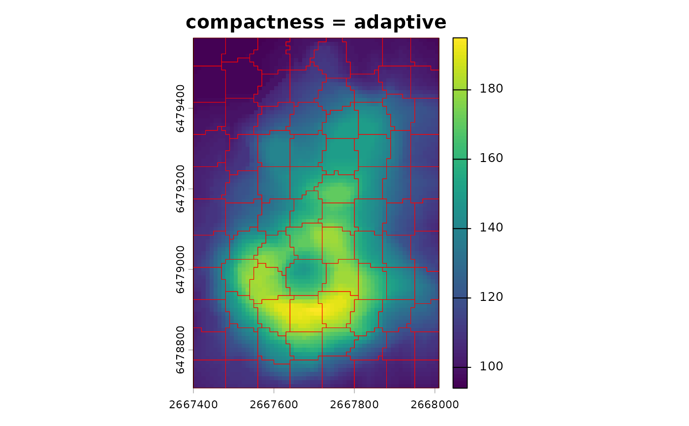

When you compare results, keep in mind that metrics from adaptive compactness are not directly comparable to fixed-compactness runs. You can still compare spatial metrics, but value metrics reflect local scaling when compactness = use_adaptive().

Manual tuning

A parallel approach to deciding on compactness is to run a small grid of values and compare the global metrics. It allows you to see the tradeoffs between spatial and value distances across a range of compactness settings.

cmp_vals <- c(1, 3, 5, 8)
cmp_metrics <- lapply(cmp_vals, function(cmp) {
  sc_i <- sc_slic(vol, step = 8, compactness = cmp)
  sc_metrics_global(vol, sc_i, scale = TRUE)
})
cmp_metrics <- do.call(rbind, cmp_metrics)
cmp_metrics
#>   step compactness adaptive_method n_supercells mean_spatial_dist_scaled
#> 1    8           1            <NA>           90                0.5500066
#> 2    8           3            <NA>           88                0.5246759
#> 3    8           5            <NA>           89                0.4982282
#> 4    8           8            <NA>           88                0.4610799
#>   mean_value_dist_scaled mean_combined_dist    balance
#> 1              2.1412253          2.3003626  1.1923986
#> 2              0.7473867          0.9994451  0.2193843
#> 3              0.4746065          0.7533578 -0.1505373
#> 4              0.3358298          0.6175536 -0.4145741

Distance and averaging functions

The dist_fun argument defines how similarity is measured in value space. Built-in options include "euclidean", Jensen–Shannon divergence, and dynamic time warping. You can also pass a name of the distance measure from the philentropy package¹ or a custom function that takes two numeric vectors and returns a single number. If you use a custom distance, ensure it returns a single finite number.

sc_manhattan <- sc_slic(vol, step = 8, compactness = 5, dist_fun = "manhattan")

The avg_fun argument controls how values are summarized within each supercell. The SLIC algorithm iteratively updates supercell centers based on the average value of the assigned pixels – and with this argument you can choose how that average is calculated. The default is "mean", and "median" is an alternative, often more robust to outliers.

sc_median <- sc_slic(vol, step = 8, compactness = 5, avg_fun = "median")

terra::plot(vol, main = "dist_fun = manhattan")
plot(sf::st_geometry(sc_manhattan), add = TRUE, border = "red", lwd = 0.5)
terra::plot(vol, main = "avg_fun = median")
plot(sf::st_geometry(sc_median), add = TRUE, border = "red", lwd = 0.5)

If you change dist_fun or avg_fun, you should remember to update compactness. Different distances change the scale of value differences and therefore the balance with the spatial term.

After tuning, use sc_metrics_pixels(), sc_metrics_supercells(), or sc_metrics_global() to compare runs. These functions accept the raster as x and the supercells as sc, and they reuse the stored dist_fun when available. See the evaluation vignette for guidance on interpreting these metrics: https://jakubnowosad.com/supercells/articles/v2-evaluation.html.

Connectivity and minimum size

The clean argument, enabled by default, enforces connectivity and removes small fragments that may arise during the iterative process of assigning pixels to supercells. This is usually desirable for polygon outputs and downstream analyses. The minarea argument sets a minimum expected size in pixels for supercells, and smaller supercells are merged into neighbors. By default, when clean = TRUE, a minimum size is still enforced internally (about one quarter of the average supercell size), so small fragments are merged unless you turn off cleaning. If you see many tiny supercells, increase minarea or step.

sc_clean <- sc_slic(vol, step = 8, compactness = 5, clean = TRUE, minarea = 20)

If you need unpostprocessed supercells for speed or debugging, you can set clean = FALSE.

Iterations

You can inspect how the algorithm converges over iterations with sc_slic_convergence(). It returns a data frame with per-iteration mean distance and has a dedicated plot() method.

sc_conv <- sc_slic_convergence(vol, step = 8, compactness = 5, iter = 10)
plot(sc_conv)

Use the diagnostics to decide whether fewer iterations are sufficient. If the curves stabilize early, you can reduce iter to speed up large runs.

Jakub Nowosad

2026-02-09